2.1 ANOVA
This summer I collected data during the fieldwork in Khodz (Koshekhablsky District, Republic of Adygea, Russia). The participants (nine native speakers of Kuban dialect of Kabardian) were asked to solve several speech production tasks:
- tell a story based on the picture to other participant
- read a prosaic text
- read a verse
Articulation rate was calculated as the number of syllables per second.
Data is here
speech_rate <- read.csv("https://goo.gl/amxSxi")
str(speech_rate)
## 'data.frame':    710 obs. of  3 variables:
##  $ dictor: Factor w/ 10 levels "all","D1","D2",..: 2 2 2 2 2 2 2 2 2 2 ...
##  $ type  : Factor w/ 3 levels "narrative","prose",..: 1 1 1 1 1 1 1 1 1 1 ...
##  $ rate  : num  2.41 3.89 3.39 3.4 2.62 ...
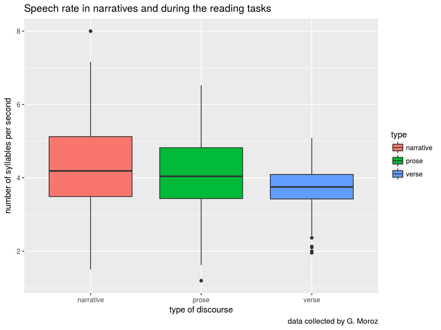
How speech rate depends on speech activity?
library(tidyverse)
speech_rate %>%
  ggplot(aes(type, rate, fill = type))+
  geom_boxplot()+
  labs(title = "Speech rate in narratives and during the reading tasks",
       caption = "data collected by G. Moroz",
       x = "type of discourse",
       y = "number of syllables per second")
We can use pairwise comparison, but … there is a Multiple comparison problem.
Anova’s H\(_0\) is that μ\(_{narrative}\) = μ\(_{prose}\) = μ\(_{verse}\)
Anova’s H\(_1\) is that μ\(_{narrative}\) ≠ μ\(_{prose}\) or μ\(_{narrative}\) ≠ μ\(_{verse}\) or μ\(_{verse}\) ≠ μ\(_{prose}\)
fit <- aov(rate~type, data = speech_rate)
summary(fit)
##              Df Sum Sq Mean Sq F value   Pr(>F)
## type          2   41.4    20.7   25.88 1.42e-11 ***
## Residuals   707  565.4     0.8
## ---
## Signif. codes:  0 '***' 0.001 '**' 0.01 '*' 0.05 '.' 0.1 ' ' 1
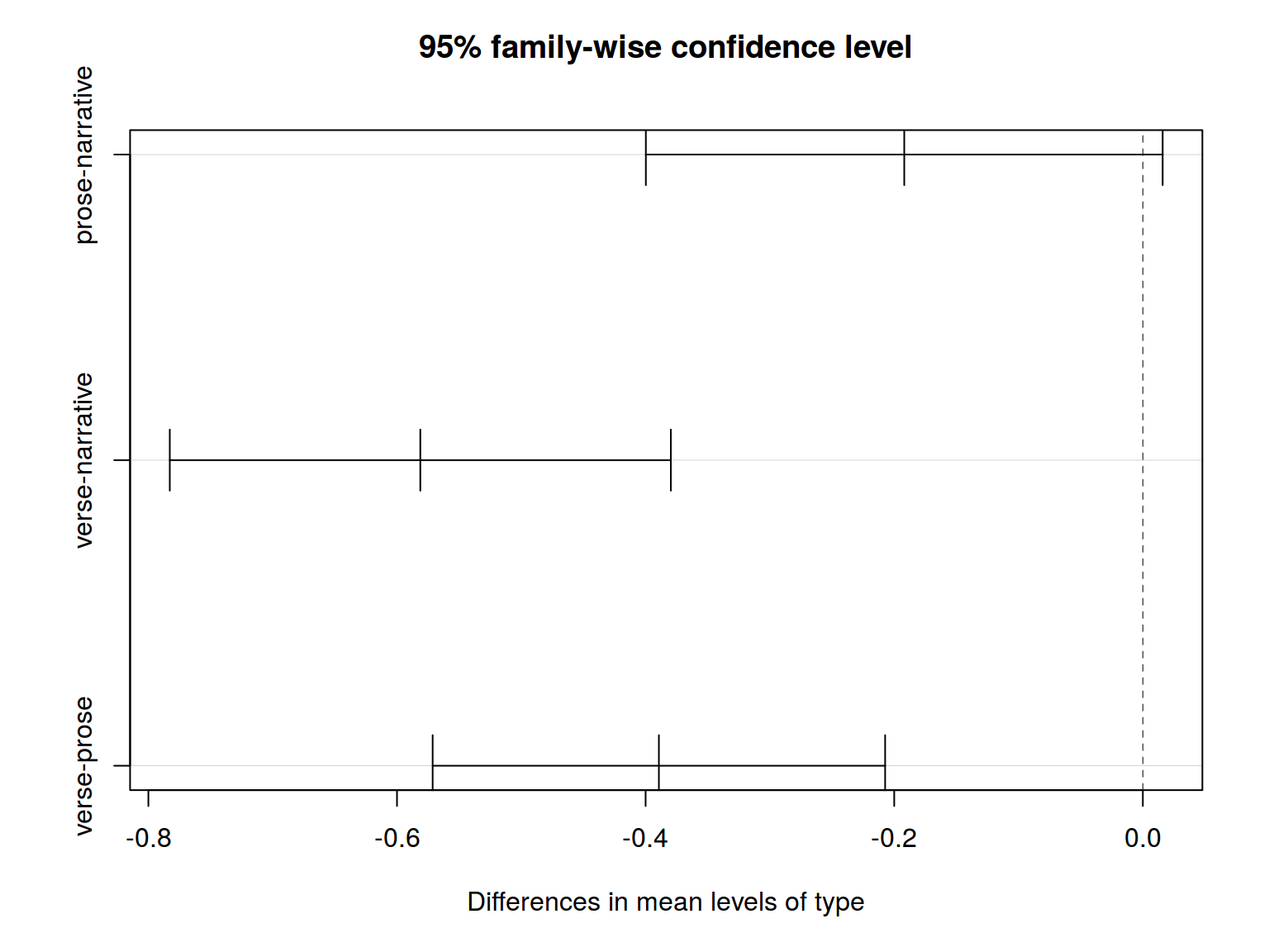
All right. There is a statistically significant result, so we can reject H\(_0\) (all groups are not simply random samples of the same population). But what the difference between them? There are a lot of different ways to understand it. We will use Tukey’s HSD (honest significant difference) test.
##   Tukey multiple comparisons of means
##     95% family-wise confidence level
##
## Fit: aov(formula = rate ~ type, data = speech_rate)
##
## $type
##                       diff        lwr         upr     p adj
## prose-narrative -0.1919299 -0.3998061  0.01594636 0.0773714
## verse-narrative -0.5812460 -0.7827826 -0.37970950 0.0000000
## verse-prose     -0.3893162 -0.5713164 -0.20731599 0.0000019
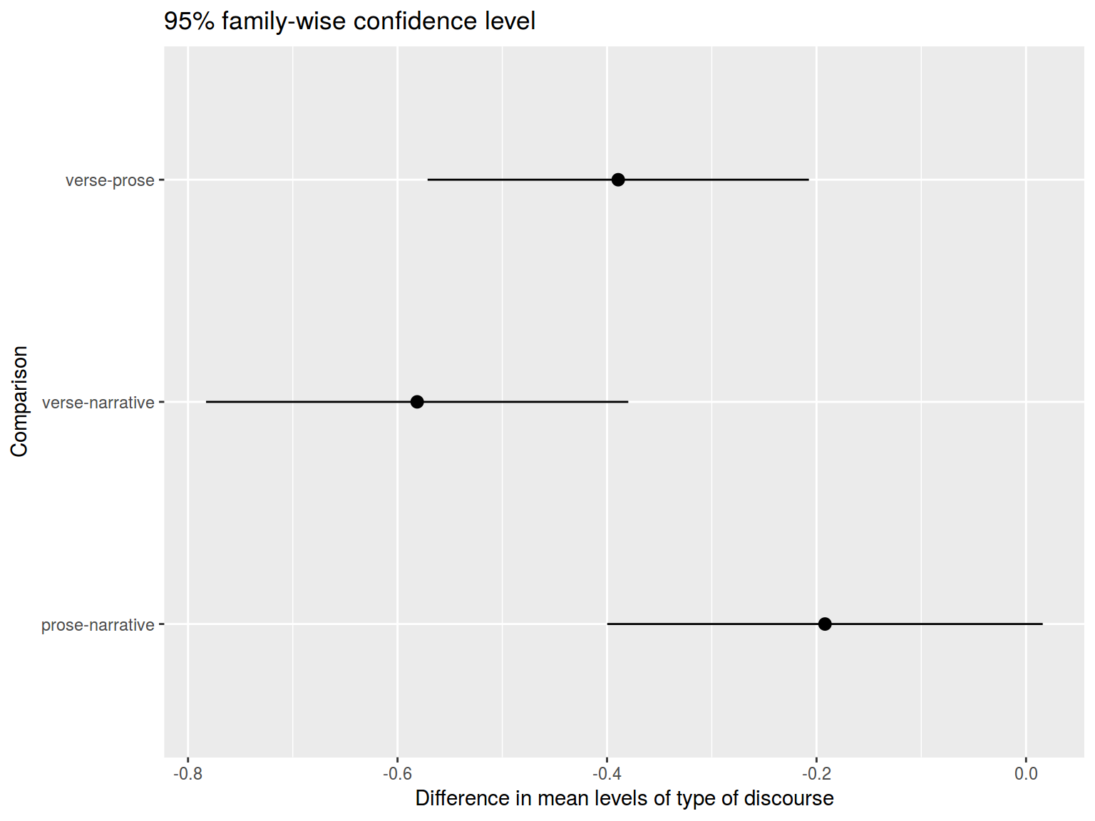
Fast visualization:
ggplot
tk <- data.frame(tk$type)
tk$Comparison <- row.names(tk)

tk %>%
  ggplot(aes(Comparison, y = diff, ymin = lwr, ymax = upr)) +
  geom_pointrange() +
  labs(title = "95% family-wise confidence level",
    y = "Difference in mean levels of type of discourse") +
  coord_flip()
3.1 Multiple linear regression
- Simple linear regression: \(y_i = \beta_0+\beta_1\times predictor_1 + \epsilon_i\)
mtcars %>%
  ggplot(aes(mpg, wt))+
  geom_smooth(method = "lm")+
  geom_point()
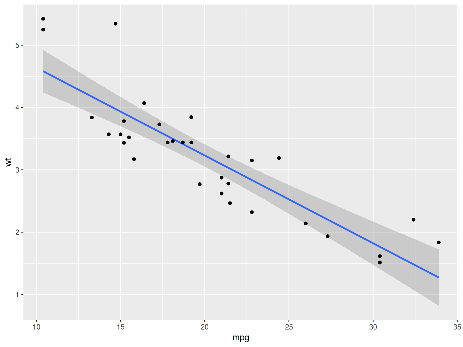
fit <- lm(mpg~wt, mtcars)
summary(fit)
##
## Call:
## lm(formula = mpg ~ wt, data = mtcars)
##
## Residuals:
##     Min      1Q  Median      3Q     Max
## -4.5432 -2.3647 -0.1252  1.4096  6.8727
##
## Coefficients:
##             Estimate Std. Error t value Pr(>|t|)
## (Intercept)  37.2851     1.8776  19.858  < 2e-16 ***
## wt           -5.3445     0.5591  -9.559 1.29e-10 ***
## ---
## Signif. codes:  0 '***' 0.001 '**' 0.01 '*' 0.05 '.' 0.1 ' ' 1
##
## Residual standard error: 3.046 on 30 degrees of freedom
## Multiple R-squared:  0.7528, Adjusted R-squared:  0.7446
## F-statistic: 91.38 on 1 and 30 DF,  p-value: 1.294e-10
- Multiple linear regression: \(y_i = \beta_0+\beta_1\times predictor_1 + ... + \beta_k\times predictor_k + \epsilon_i\)
fit2 <- lm(mpg~wt+hp, mtcars)
summary(fit2)
##
## Call:
## lm(formula = mpg ~ wt + hp, data = mtcars)
##
## Residuals:
##    Min     1Q Median     3Q    Max
## -3.941 -1.600 -0.182  1.050  5.854
##
## Coefficients:
##             Estimate Std. Error t value Pr(>|t|)
## (Intercept) 37.22727    1.59879  23.285  < 2e-16 ***
## wt          -3.87783    0.63273  -6.129 1.12e-06 ***
## hp          -0.03177    0.00903  -3.519  0.00145 **
## ---
## Signif. codes:  0 '***' 0.001 '**' 0.01 '*' 0.05 '.' 0.1 ' ' 1
##
## Residual standard error: 2.593 on 29 degrees of freedom
## Multiple R-squared:  0.8268, Adjusted R-squared:  0.8148
## F-statistic: 69.21 on 2 and 29 DF,  p-value: 9.109e-12
4.1 Variable Types
How to make numeric-to-categorical conversion?
a <- sin(1:100) # Create a random vector
b <- c(-1, -0.5, 0, 0.5, 1) # Create a vector of boundaries
table(cut(a, breaks = b))
##
## (-1,-0.5]  (-0.5,0]   (0,0.5]   (0.5,1]
##        35        15        16        34
# if the intervals should be closed on the right
table(cut(a, breaks = b, right = F))
##
## [-1,-0.5)  [-0.5,0)   [0,0.5)   [0.5,1)
##        35        15        16        34
How to make categorical-to-numeric conversion? Dummy variables!
4.2 Dummy variables
Dummy variable it is a technique for creating a numeric variable from categorical. For each \(n-1\) levels of a categorical variable it creates a dummy variable, which have value 1 for certain level of variable and 0 otherwise.
sex variable with 2 levels can be replaced with 1 dummy variable sex_female:
- sex_female = 1, if an individual is a female
- sex_female = 0, if an individual is a female, then
Eye color variable with 4 levels (blue, brown, gray, green) can be replaced with 3 dummy variables
- eye_blue = 1, if an eye variable is blue; otherwise — 0
- eye_brown = 1, if an eye variable is brown; otherwise — 0
- eue_gray = 1, if an eye variable is gray; otherwise — 0
- green value of eye variable is coded as 0 value of all eye_blue, eye_brown and eye_grey variables.
| blue |
1 |
0 |
0 |
| brown |
0 |
1 |
0 |
| gray |
0 |
0 |
1 |
| green |
0 |
0 |
0 |
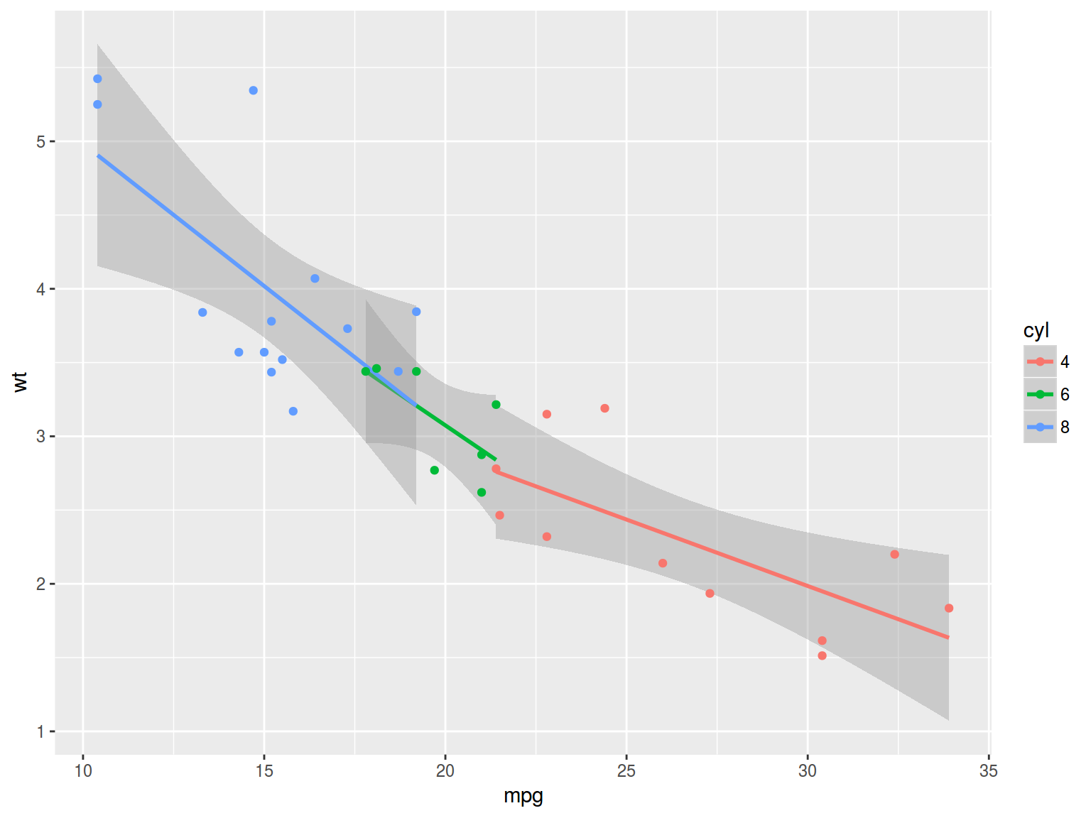
4.3 Regression example
mtcars %>%
  mutate(cyl = factor(cyl)) %>%
  ggplot(aes(mpg, wt, color = cyl))+
  geom_smooth(method = "lm")+
  geom_point()
fit2 <- lm(mpg~wt+factor(cyl), mtcars)
summary(fit2)
##
## Call:
## lm(formula = mpg ~ wt + factor(cyl), data = mtcars)
##
## Residuals:
##     Min      1Q  Median      3Q     Max
## -4.5890 -1.2357 -0.5159  1.3845  5.7915
##
## Coefficients:
##              Estimate Std. Error t value Pr(>|t|)
## (Intercept)   33.9908     1.8878  18.006  < 2e-16 ***
## wt            -3.2056     0.7539  -4.252 0.000213 ***
## factor(cyl)6  -4.2556     1.3861  -3.070 0.004718 **
## factor(cyl)8  -6.0709     1.6523  -3.674 0.000999 ***
## ---
## Signif. codes:  0 '***' 0.001 '**' 0.01 '*' 0.05 '.' 0.1 ' ' 1
##
## Residual standard error: 2.557 on 28 degrees of freedom
## Multiple R-squared:  0.8374, Adjusted R-squared:   0.82
## F-statistic: 48.08 on 3 and 28 DF,  p-value: 3.594e-11