- Введение в R и визуализация данных
Г. Мороз
Презентация доступна по ссылке: goo.gl/78y9br
0. Как добыть R и Rstudio
Бесплатное программное обеспечение:
1. Основы R
1.1 Базовые элементы
9L # целое число## [1] 9-3.47 # рациональные числа## [1] -3.475+2i # мнимое число## [1] 5+2i"Санкт-Петербург" # строка## [1] "Санкт-Петербург"TRUE # логическое значение## [1] TRUEFALSE # логическое значение## [1] FALSEpi # число π## [1] 3.1415931.2 Калкулятор
2+2## [1] 49-4.5## [1] 4.5117*2## [1] 234234/2## [1] 1175^7## [1] 781255**7## [1] 7812525^0.5## [1] 525^(1/2) # скобки!## [1] 525^1/2 # скобки!## [1] 12.555%%3 # остаток от деления## [1] 1sin(pi/2)## [1] 1cos(pi)## [1] -1sum(34, 23, 14)## [1] 71prod(34, 23, 14)## [1] 109481.3 Векторы и его индексация
2:9## [1] 2 3 4 5 6 7 8 933:25## [1] 33 32 31 30 29 28 27 26 25-5:-3## [1] -5 -4 -3c(1,5,8,3)## [1] 1 5 8 3rep(c(8, 2), 4)## [1] 8 2 8 2 8 2 8 2rep(c(8, 2), each = 4)## [1] 8 8 8 8 2 2 2 2c(TRUE, TRUE, FALSE, TRUE)[4]## [1] TRUEc("alpha", "beta", "gamma")[2:3]## [1] "beta" "gamma"c("alpha", "beta", "gamma")[-3]## [1] "alpha" "beta"
(1) Прибавьте к вектору
1:54
(2) Посчитайте \[\frac{\sum_{i=1}^{100}4 \times i^2}{1250}\]
1.4 Переменные
a <- 5:24 # Сочетание Alt - ставит стрелочку
a[3]
## [1] 7a <- a + 3
a[3]## [1] 1023 -> a
a## [1] 23letters## [1] "a" "b" "c" "d" "e" "f" "g" "h" "i" "j" "k" "l" "m" "n" "o" "p" "q"
## [18] "r" "s" "t" "u" "v" "w" "x" "y" "z"LETTERS## [1] "A" "B" "C" "D" "E" "F" "G" "H" "I" "J" "K" "L" "M" "N" "O" "P" "Q"
## [18] "R" "S" "T" "U" "V" "W" "X" "Y" "Z"a == 23 # равно?## [1] TRUEa != 28 # не равно?## [1] TRUEb <- 1:30
b[b %% 3 == 0] # индекс принимает условие!## [1] 3 6 9 12 15 18 21 24 27 30
1.5 Функции и описательные статистики
height <- c(1, 1.7, 1.8, 1.74, 1.56, 1.66, 1.68, 1.77, 1.76, 6)
mean(height)
## [1] 2.067mean(height, trim = 0.1)## [1] 1.70875weighted.mean(height, w = c(1,2,2,2,1,2,2,1,1,1))## [1] 1.95range(height)## [1] 1 6max(height)## [1] 6min(height)## [1] 1sd(height)## [1] 1.401381median(height)## [1] 1.72quantile(height)## 0% 25% 50% 75% 100%
## 1.0000 1.6650 1.7200 1.7675 6.0000quantile(height, probs = c(0.1, 0.2))## 10% 20%
## 1.504 1.640IQR(height) # разность 3ей и 2ой квартилей## [1] 0.1025summary(height)## Min. 1st Qu. Median Mean 3rd Qu. Max.
## 1.000 1.665 1.720 2.067 1.768 6.000
1.6 Датафрейм и его индексация
df <- data.frame(name = c("a", "b", "c", "d", "f"),
           height = c(1.76, 1.56, 1.45, 1.94, 1.81),
           brown_hair = c(FALSE, TRUE, FALSE, TRUE, TRUE))
dfhead(df)tail(df)summary(df)## name height brown_hair
## a:1 Min. :1.450 Mode :logical
## b:1 1st Qu.:1.560 FALSE:2
## c:1 Median :1.760 TRUE :3
## d:1 Mean :1.704
## f:1 3rd Qu.:1.810
## Max. :1.940df[1,]df[,2]## [1] 1.76 1.56 1.45 1.94 1.81df$name## [1] a b c d f
## Levels: a b c d f1.7 Считывание файлов в R
df <- read.table("путь к файлу")
df <- read.table("интернет ссылка")
df <- read.table(...) # разделитель: запятая
df <- read.table(..., sep = "\t") # разделитель: табуляция
df <- read.table(..., sep = ";") # разделитель: точка с запятой
1.8 Работа с пакетами
install.packages("ggplot2") #  установить пакет
library("ggplot2") #  включить пакет
2. Визуализация в R: ggplot2
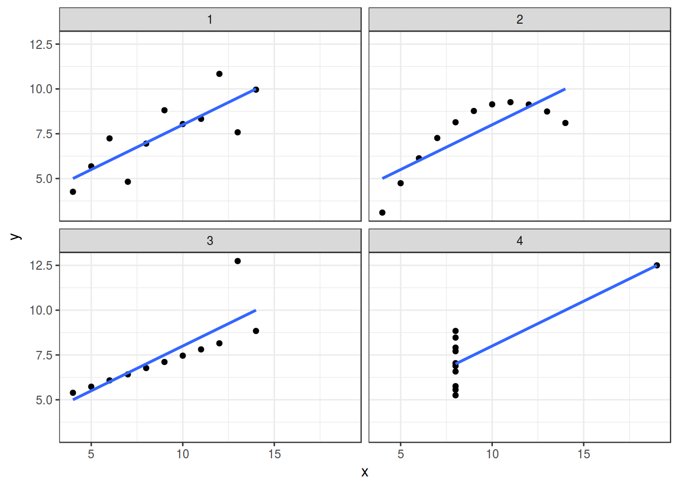
2.1.1 Почему визуализация? Anscombe’s quartet
В работе Anscombe, F. J. (1973). “Graphs in Statistical Analysis” представлены следующие данные:
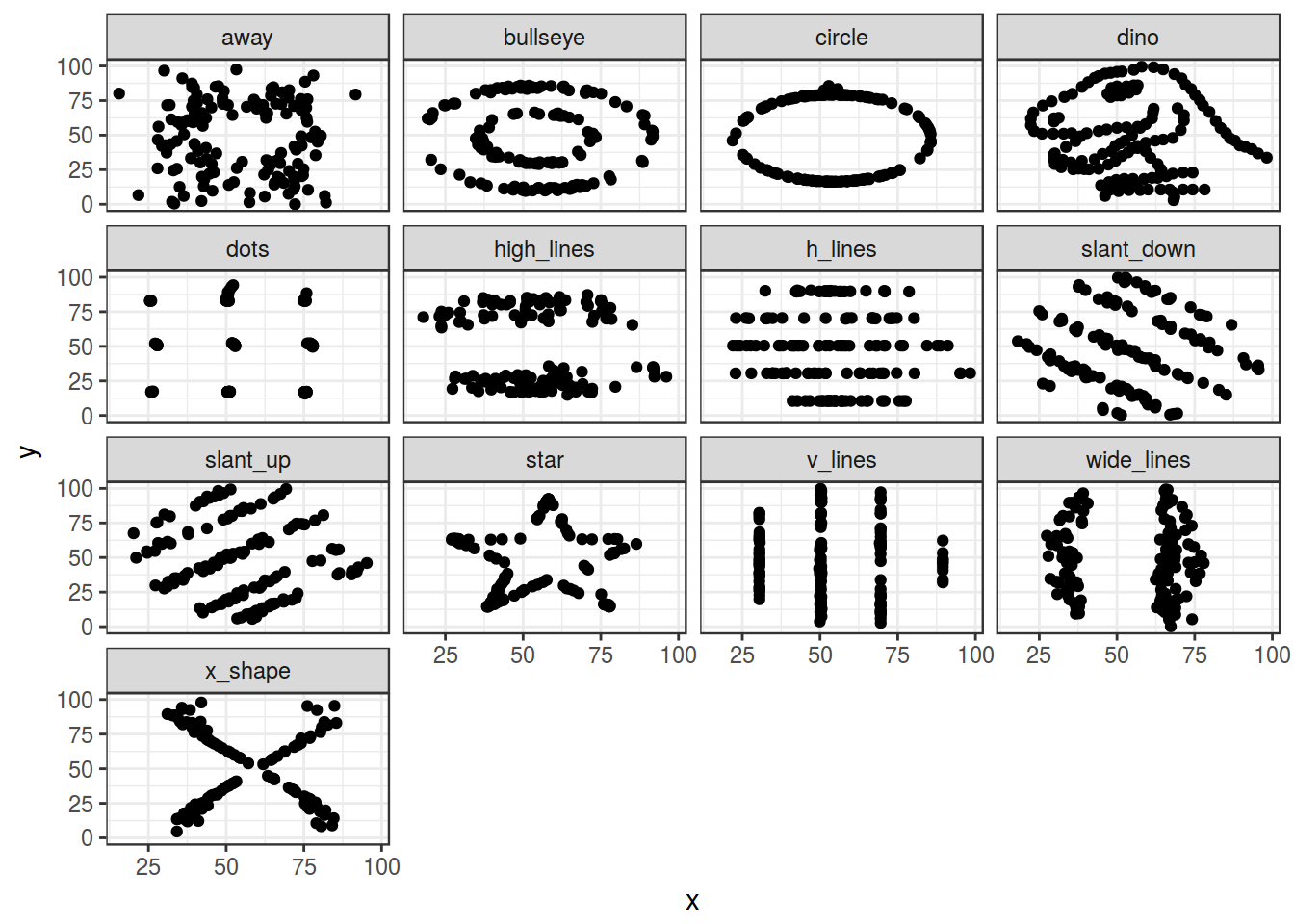
2.1.2 Почему визуализация? Datasaurus
В раблоте Matejka and Fitzmaurice (2017) “Same Stats, Different Graphs” представлены следующие данные:
2.2 Данные
Дальше все примеры будут приводится на основании результатов работы Chi-kuk 2007. В эксперименте проверялась связь акустических мер и результатов перцептивного восприятия сексуальной ориентации. Носителей кантонского диалекта китайского языка попросили послушать записи носителей кантонского диалекта и оценить ориентацию тех, кого они слушали. В датасете 14 носителей и следующие переменные:
- длительность [s] (s.duration.ms)
- длительность гласного (vowel.duration.ms)
- среднее значение частоты основного тона (average.f0.Hz)
- разброс значений частоты основного тона (f0.range.Hz)
- доля оценок как гомосексуала (perceived.as.homo)
- доля оценок как гетеросексуала (perceived.as.hetero)
- ориентация носителей (orientation)
- возраст носителей (age)
Скачиваем данные:
homo <- read.csv("http://goo.gl/Zjr9aF")
homo
Предлагаю пробовать повторять все примеры с другим датасетом, представленным М. Даниэлем. Это данные из интервью с носителями одного из северных диалектов селения Устья. В датасете 62 носителя и следующие переменные:
- год рождения (year)
- пол (gender)
- количество консервативных употреблений (cons)
- количество инновационных употреблений (inn)
- количество всех употреблений (total)
ustya <- read.csv("https://goo.gl/FqsqSX", sep = "\t")
ustya
2.3.1 Scaterplot
ggplot(data = homo, aes(s.duration.ms, vowel.duration.ms)) +
  geom_point()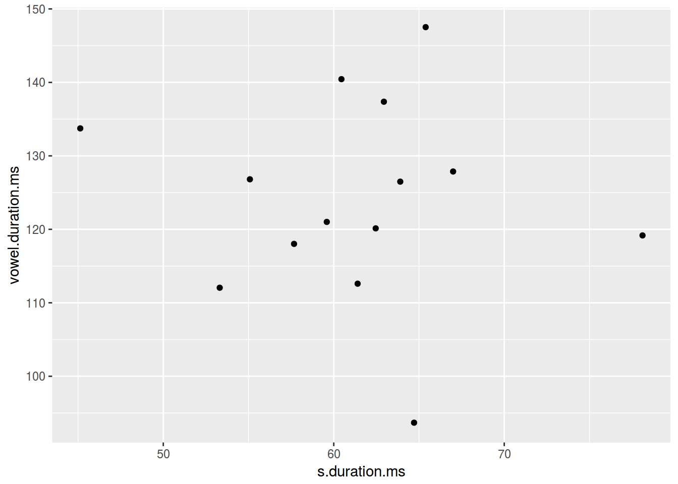
2.3.2 Scaterplot: цвет
ggplot(data = homo, aes(s.duration.ms, vowel.duration.ms,
                        color = orientation)) +
  geom_point()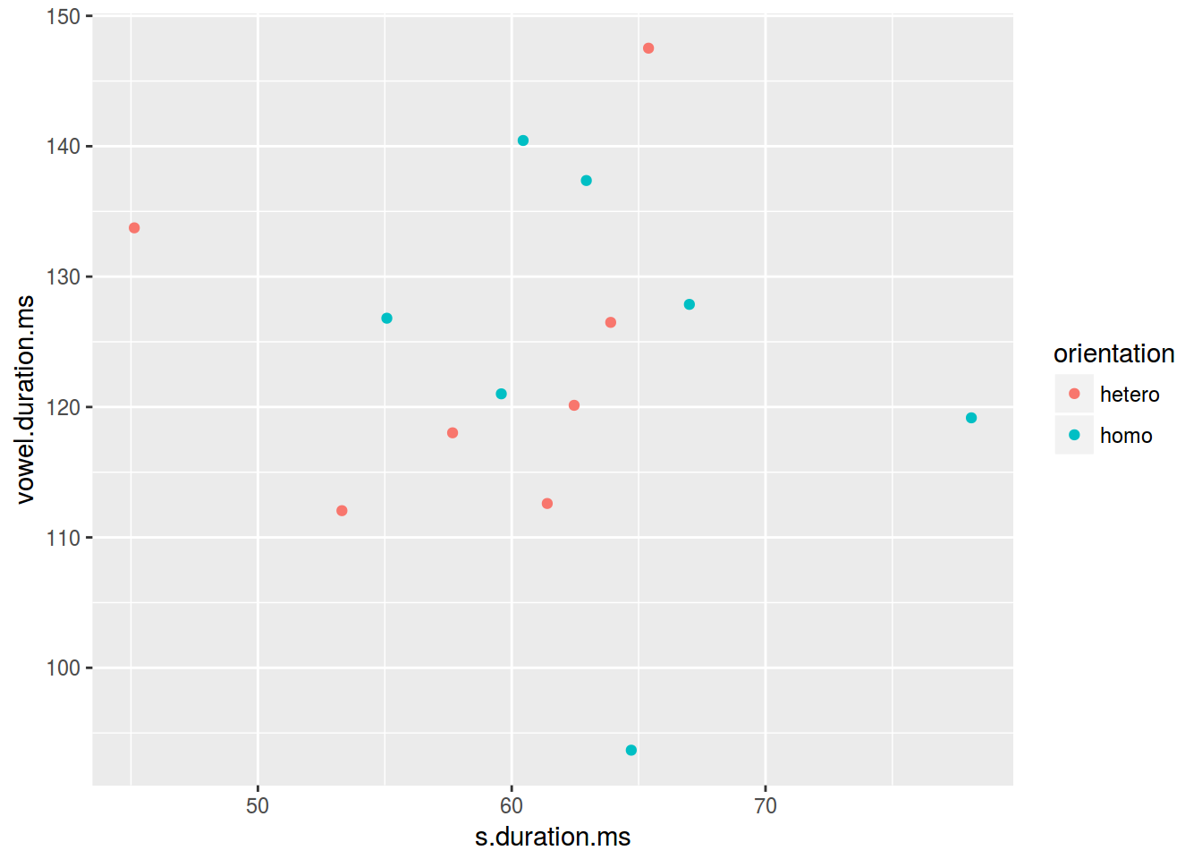
2.3.3 Scaterplot: форма
ggplot(data = homo, aes(s.duration.ms, vowel.duration.ms,
                        shape = orientation)) +
  geom_point(color = "darkgreen")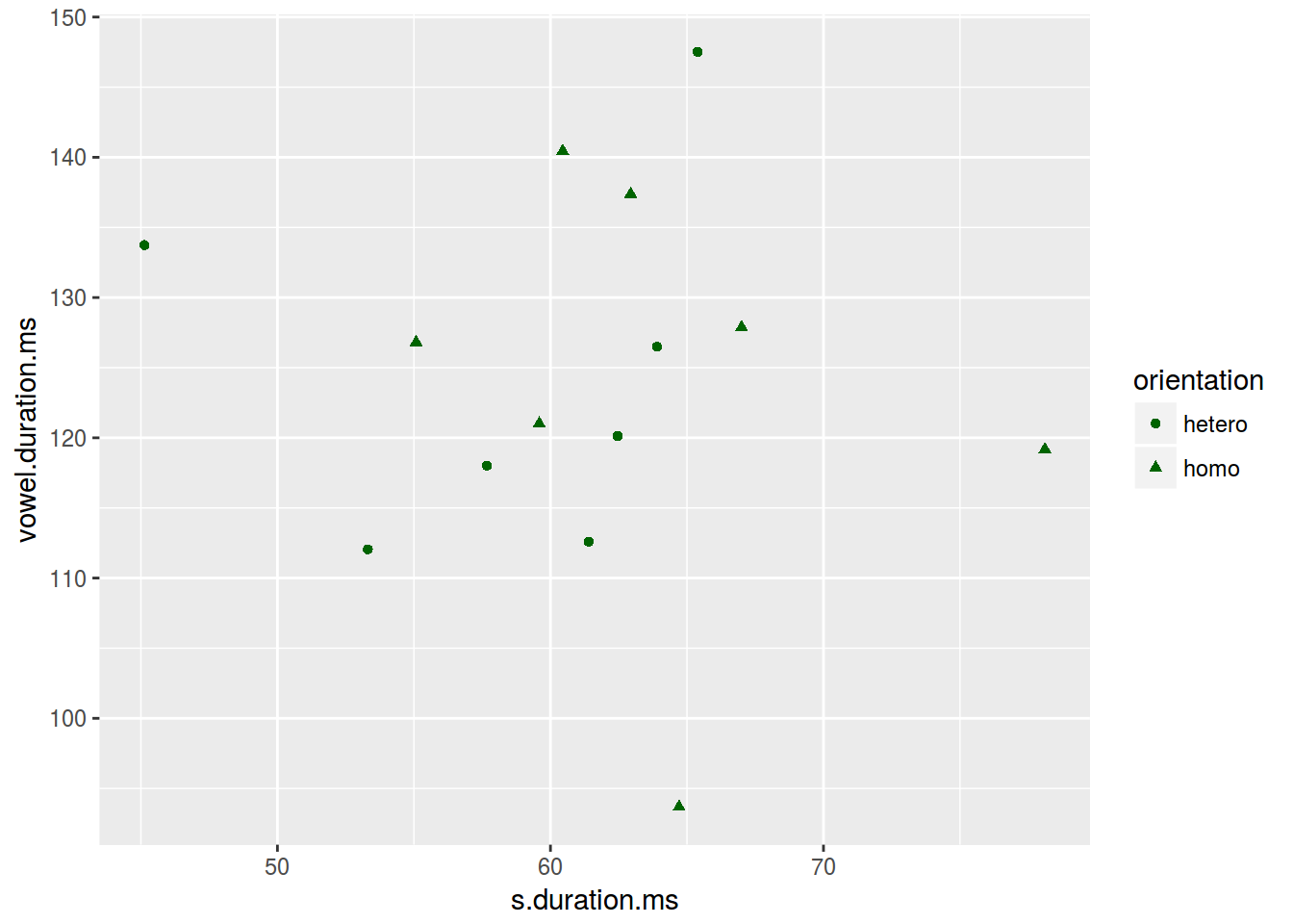
2.3.4 Scaterplot: размер
ggplot(data = homo, aes(s.duration.ms, vowel.duration.ms,
                        size = age)) +
  geom_point()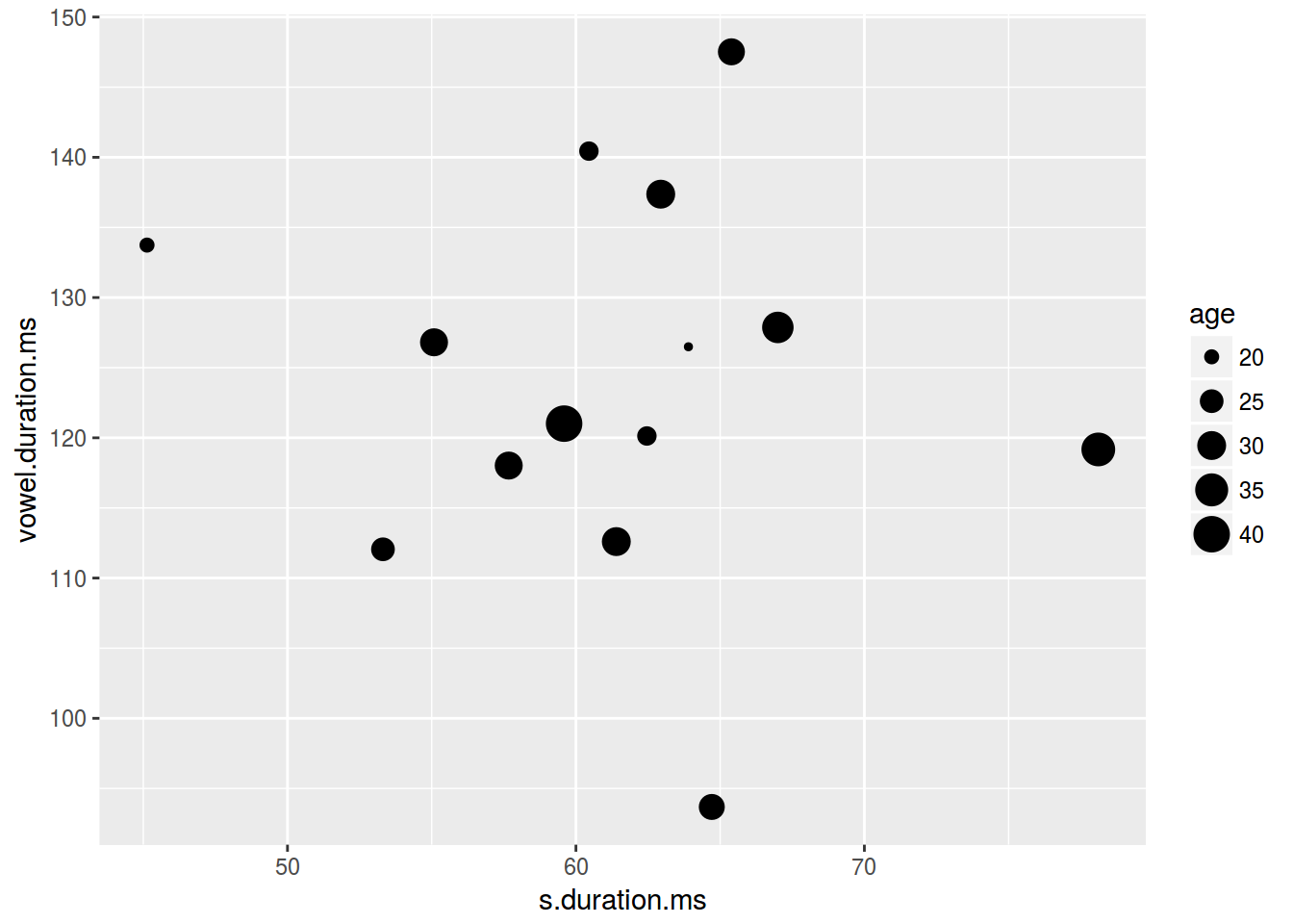
2.3.5 Scaterplot: текст
levels(homo$orientation) <- c("⚣", "⚤")
ggplot(data = homo, aes(s.duration.ms, vowel.duration.ms,
                        label = orientation, fill = orientation)) +
  geom_label()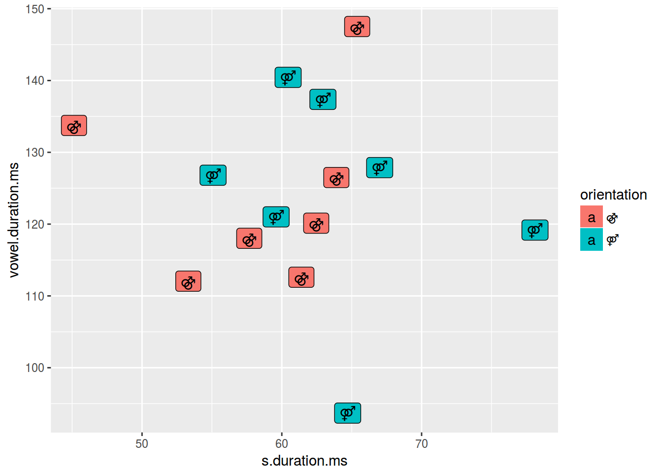
ggplot(data = homo, aes(s.duration.ms, vowel.duration.ms,
                        label = orientation, fill = orientation)) +
  geom_text()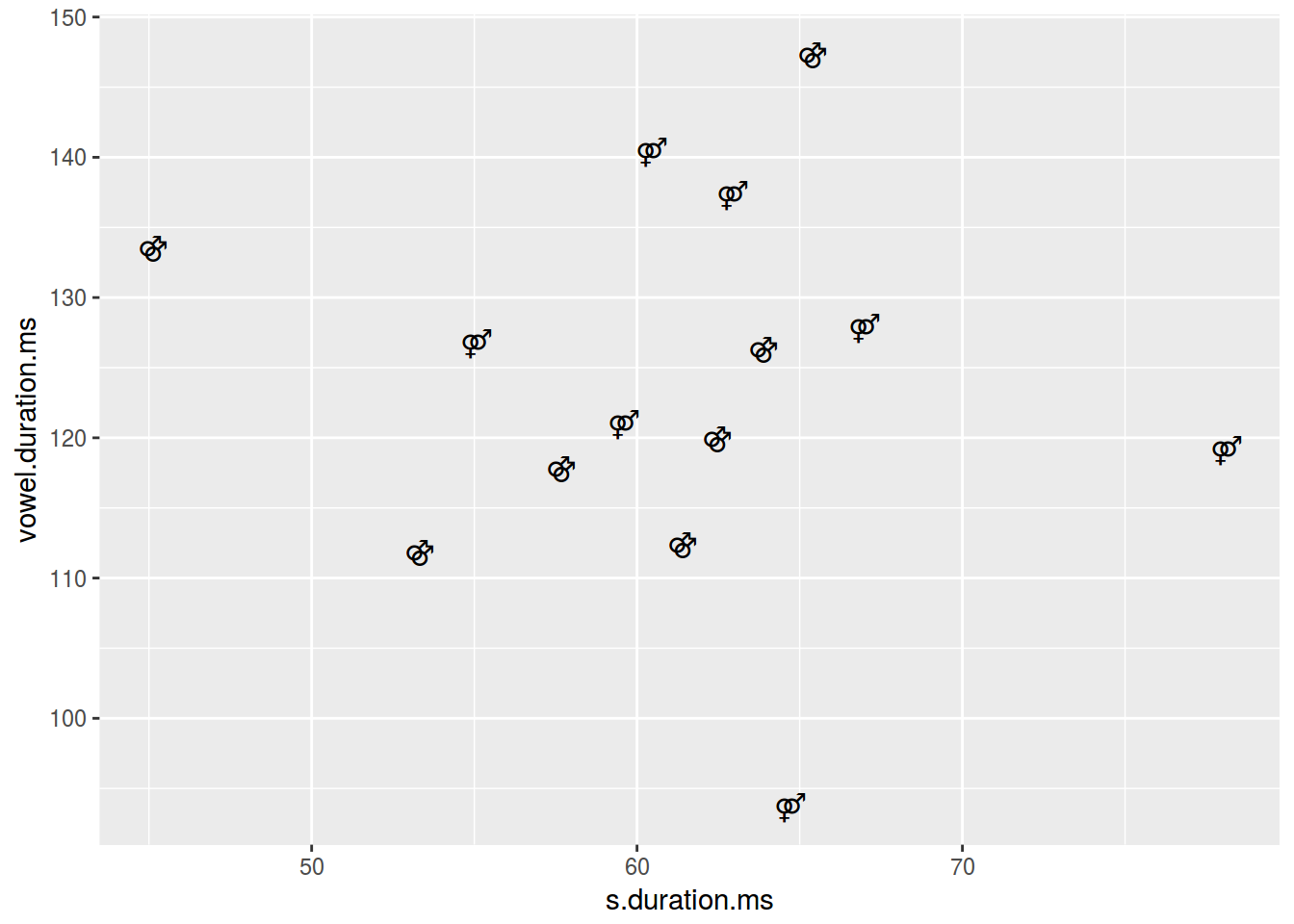
#  Но для дальнейшей лекции имеет смысл вернуть обратно.
levels(homo$orientation) <- c("homo", "hetero")
2.3.6 Scaterplot: заголовки
ggplot(data = homo, aes(s.duration.ms, vowel.duration.ms)) +
  geom_point()+
  labs(title = "length of [s] vs. length of vowels",
       subtitle = "based on 14 speakers of Cantonese",
       caption = "data from [Chi kuk 2007]")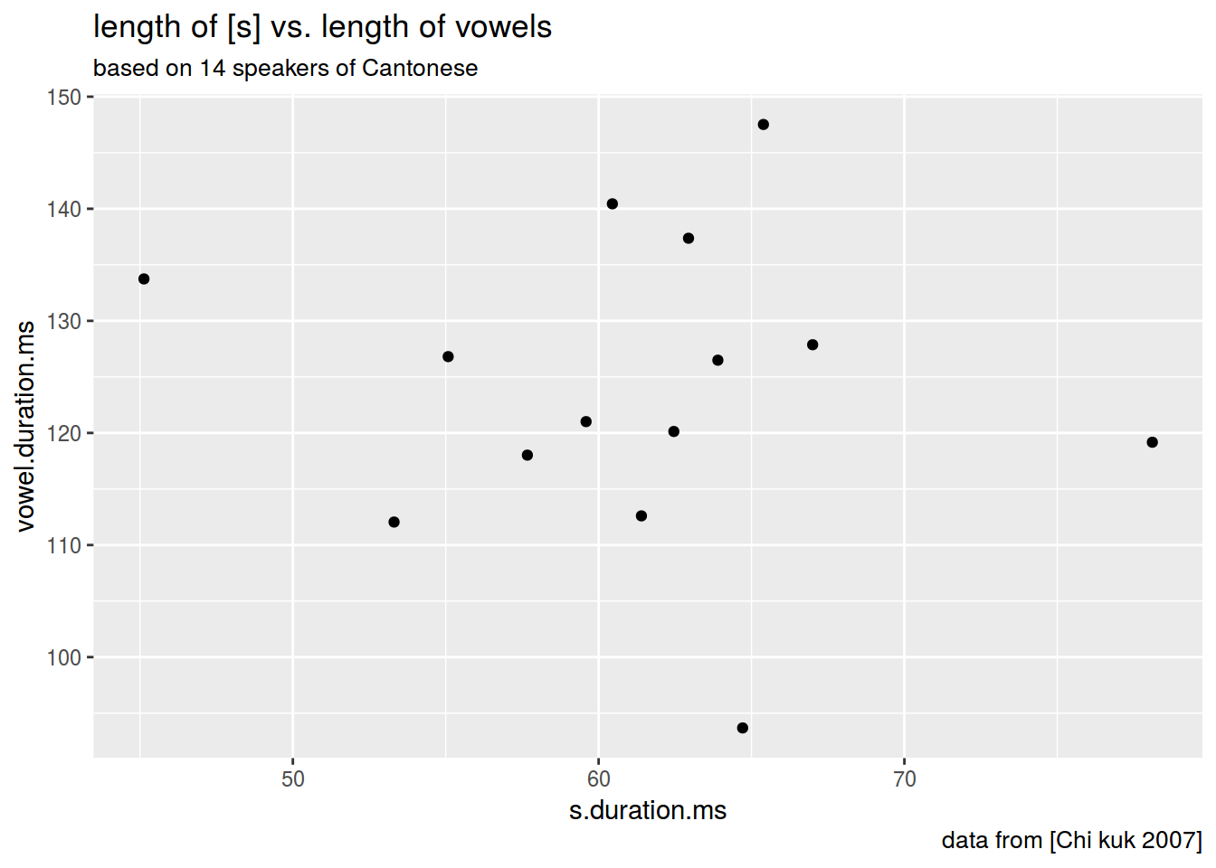
2.3.7 Scaterplot: оси
ggplot(data = homo, aes(s.duration.ms, vowel.duration.ms)) +
  geom_point()+
  xlab("duration of [s] in ms")+
  ylab("vowel duration in ms")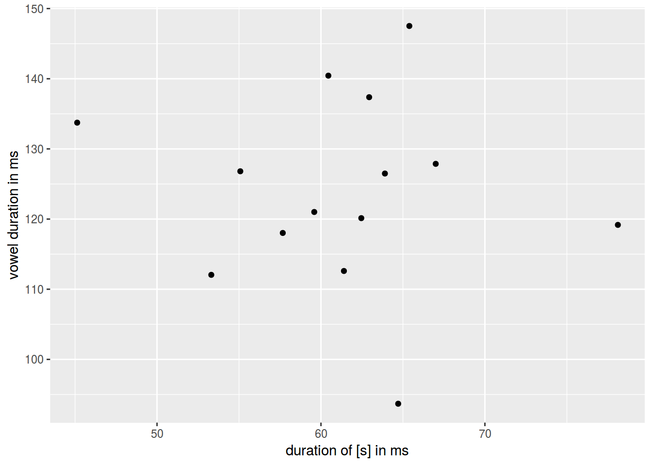
2.3.8 Scaterplot: rug
ggplot(data = homo, aes(s.duration.ms, vowel.duration.ms, color = orientation)) +
  geom_point() +
  geom_rug()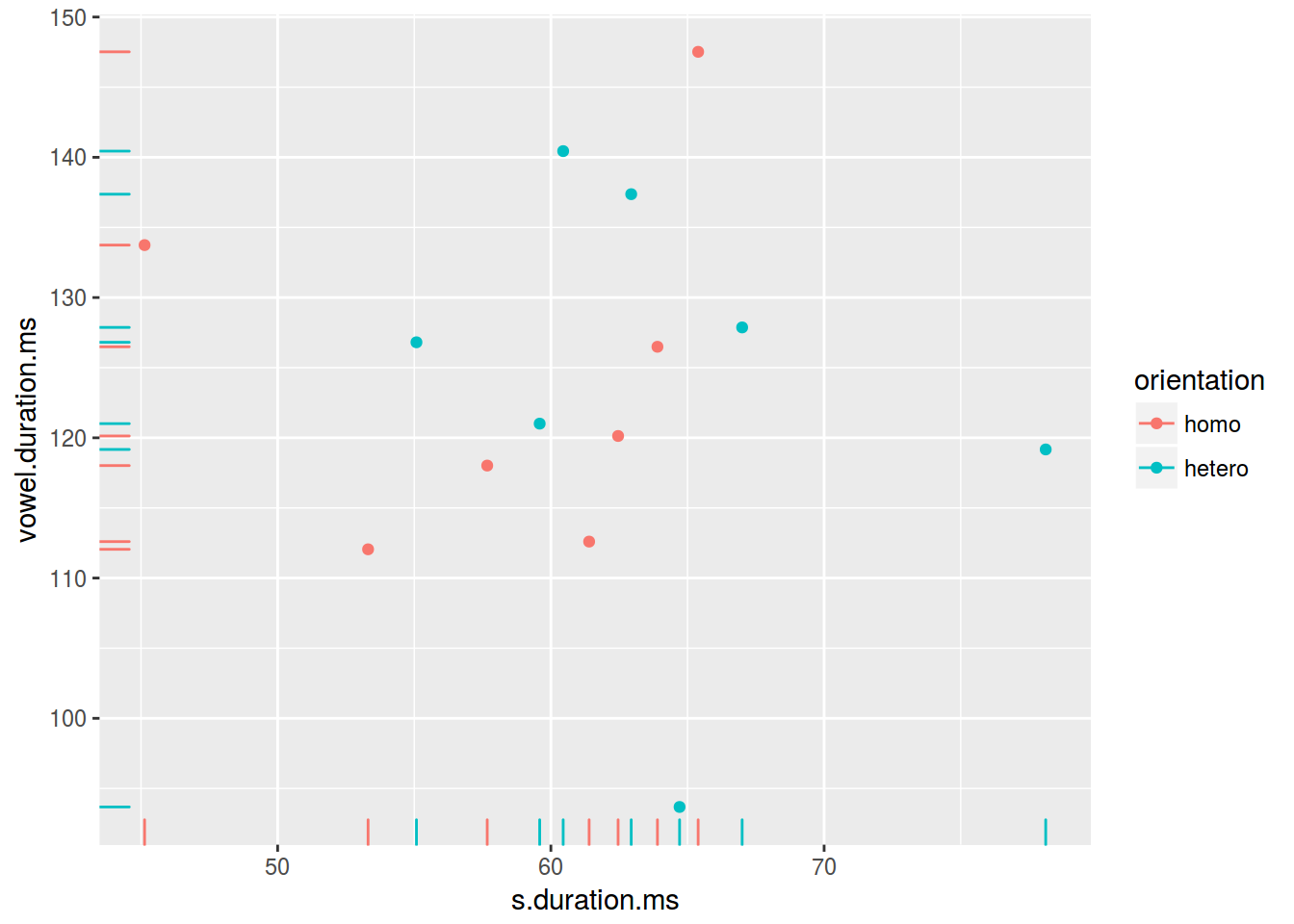
2.3.9 Scaterplot: линии
ggplot(data = homo, aes(s.duration.ms, vowel.duration.ms)) +
  geom_point() +
  geom_hline(yintercept = mean(homo$vowel.duration.ms))+
  geom_vline(xintercept = 60)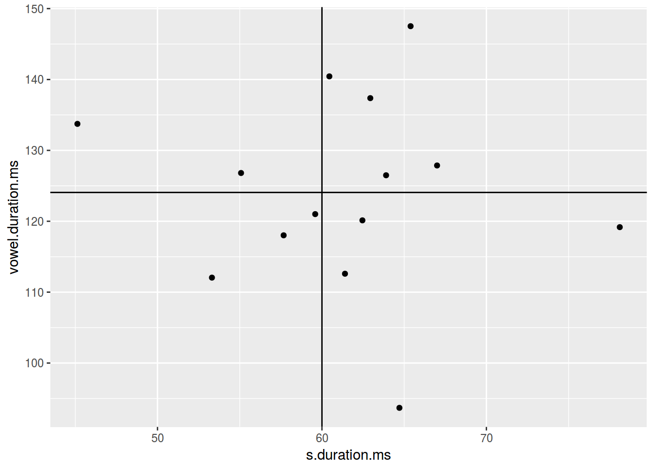
ggplot(data = homo, aes(s.duration.ms, vowel.duration.ms)) +
  geom_point() +
  geom_hline(yintercept = 120, linetype = 2)+
  geom_vline(xintercept = 60, size = 5)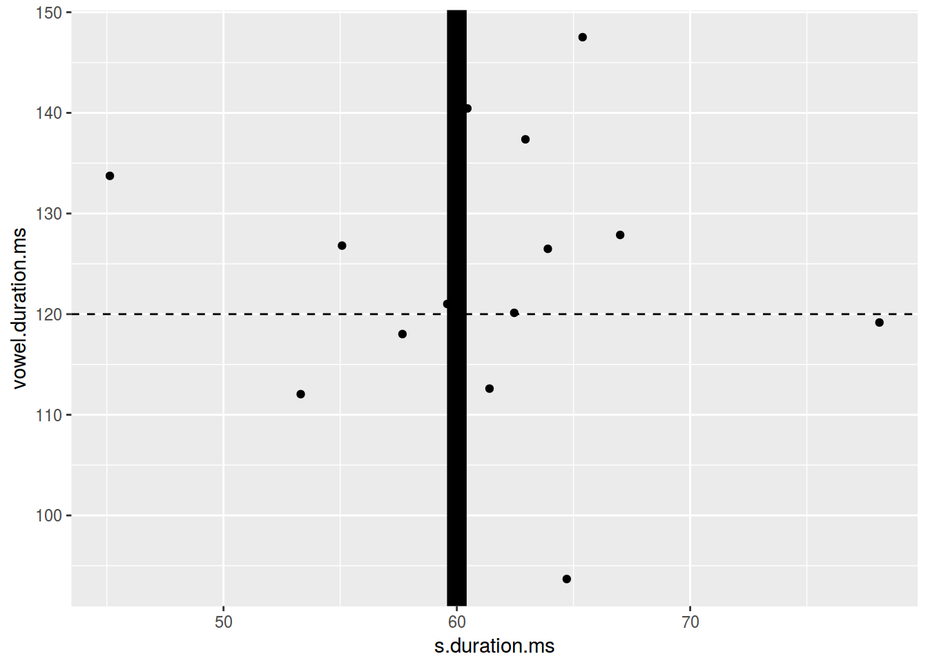
ggplot(data = homo, aes(s.duration.ms, vowel.duration.ms)) +
  geom_point() +
  geom_hline(yintercept = 120, linetype = 4)+
  geom_vline(xintercept = 60, color = "blue")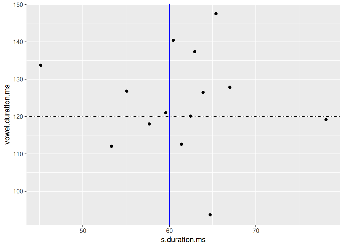
2.3.10 Scaterplot: дополнительная аннотация
The function annotate adds geoms to a plot.
ggplot(data = homo, aes(s.duration.ms, vowel.duration.ms)) +
  geom_point()+
  annotate(geom = "rect", xmin = 77, xmax = 79,
             ymin = 117, ymax = 122, fill = "red", alpha = 0.2) +
  annotate(geom = "text", x = 78, y = 125,
             label = "Who is that?\n Outlier?")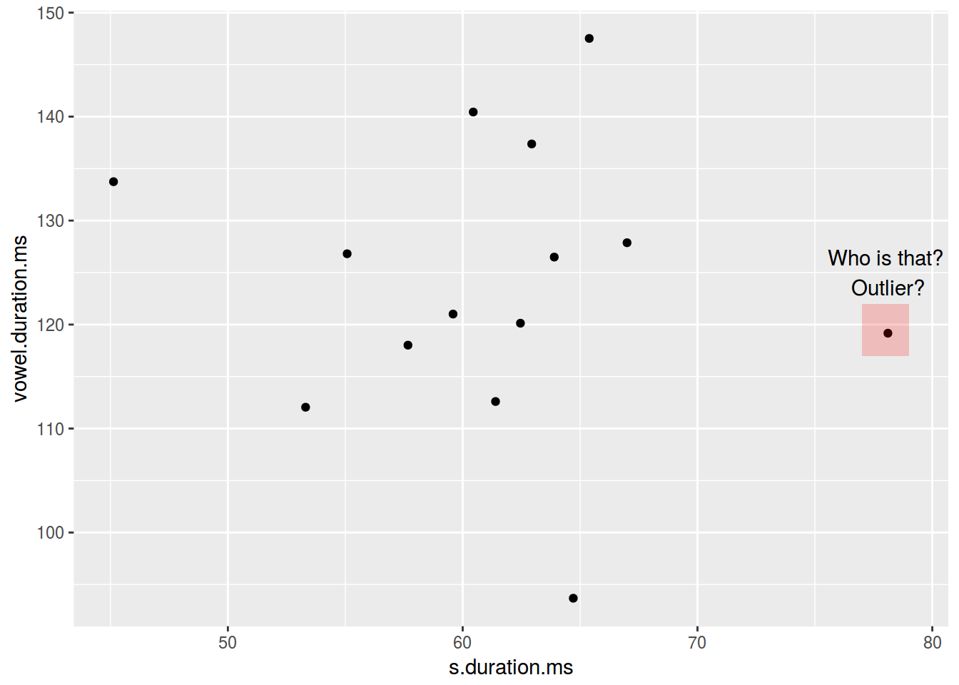
2.4.1 Barplots
Существует две возможности:
- не аггрегированные данные
head(homo[, c(1, 9)])- аггрегированные данные
head(homo[, c(1, 10)])2.4.1.1 Barplots: неаггрегированые данные
ggplot(data = homo, aes(orientation)) +
  geom_bar()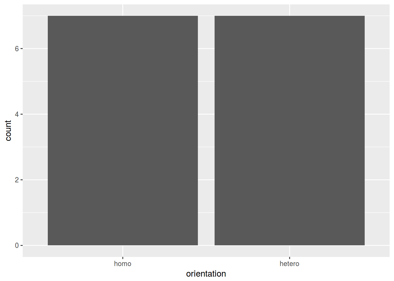
2.4.1.2 Barplots: аггрегированые данные
ggplot(data = homo, aes(speaker, age)) +
  geom_col()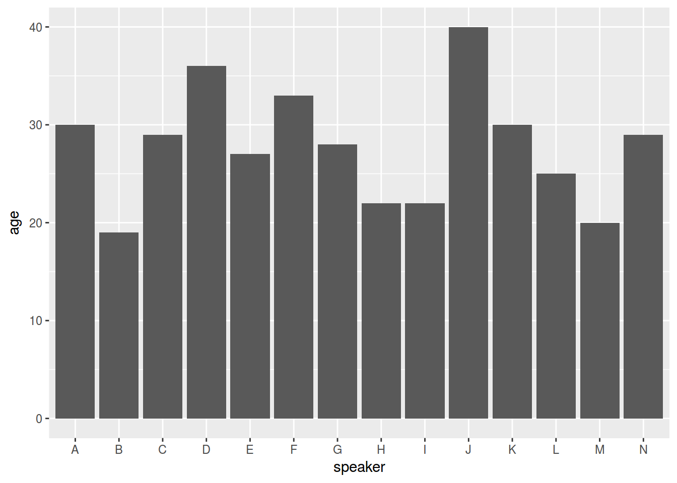
2.4.2 Barplots: цвет
ggplot(data = homo, aes(speaker, age, fill = orientation)) +
  geom_bar(stat = "identity")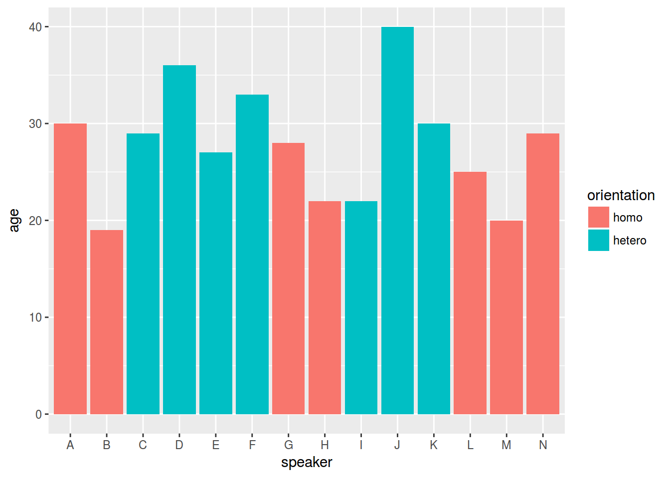
2.5.1 Ящики с усами (boxplot)
ggplot(data = homo, aes(orientation, s.duration.ms)) +
  geom_boxplot()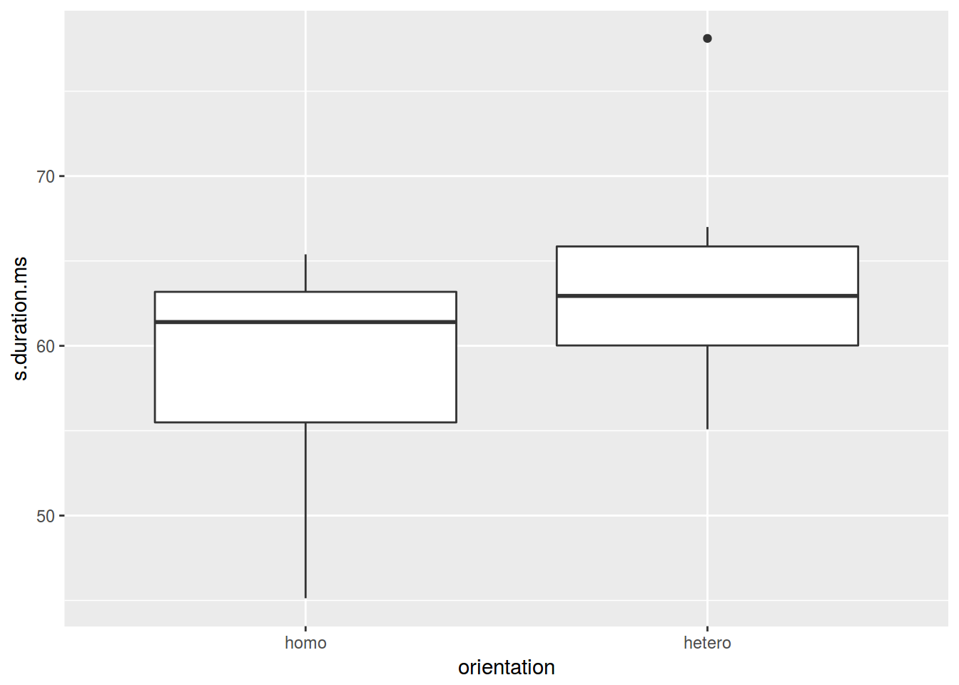
2.5.2 Ящики с усами: точки
ggplot(data = homo, aes(orientation, s.duration.ms)) +
  geom_boxplot()+
  geom_point()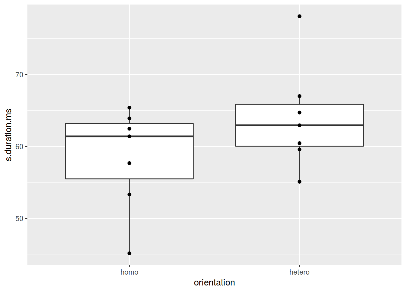
2.5.3 Ящики с усами: jitter
ggplot(data = homo, aes(orientation, s.duration.ms)) +
  geom_boxplot() +
  geom_jitter(width = 0.5)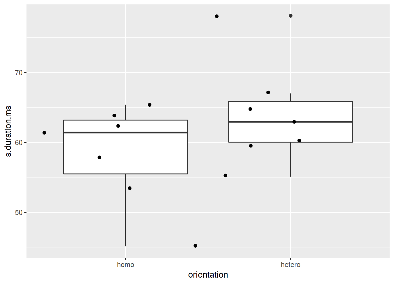
2.5.4 Violinplot
ggplot(data = homo, aes(orientation, s.duration.ms)) +
  geom_violin() +
  geom_jitter()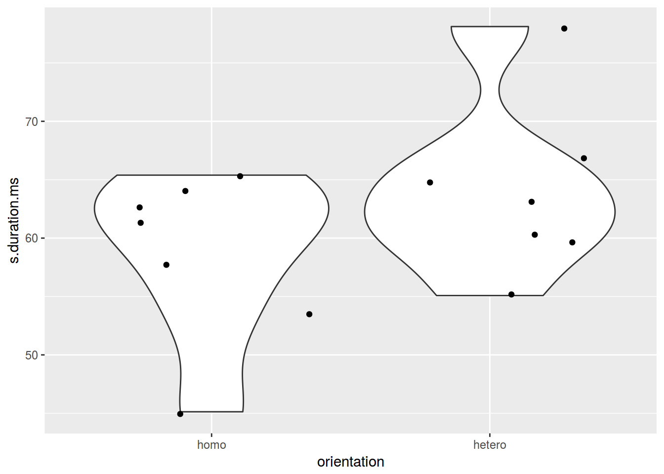
2.6.1 Гистограмма
ggplot(data = homo, aes(s.duration.ms)) +
  geom_histogram()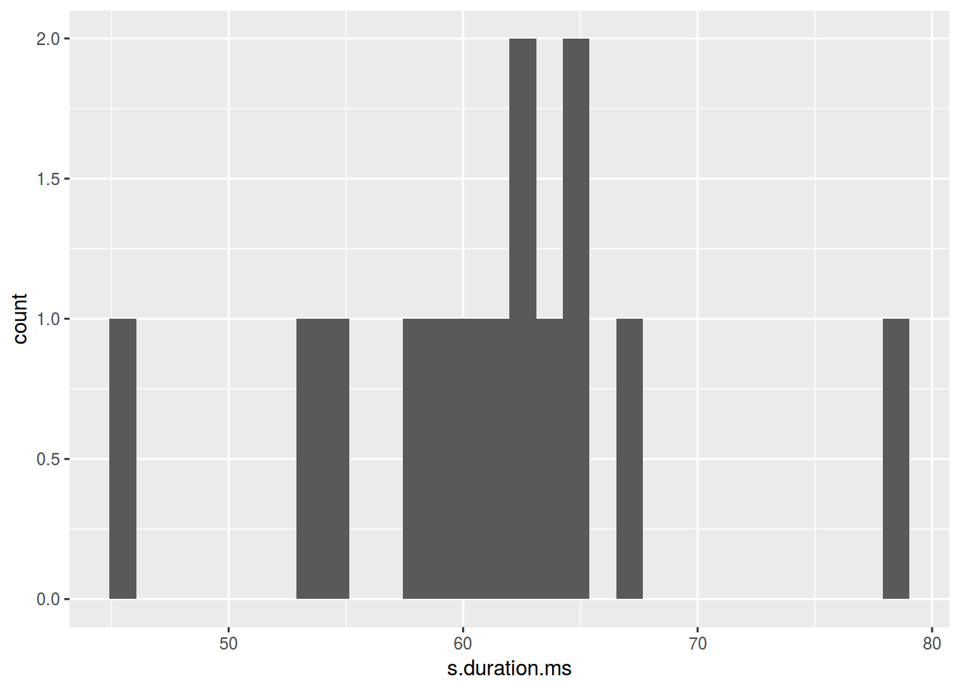
Сколько нужно ячеек?
- [Sturgers 1926] nclass.Sturges(adyghe$F1)
- [Scott 1979] nclass.scott(adyghe$F1)
- [Freedman, Diaconis 1981] nclass.FD(adyghe$F1)
ggplot(data = homo, aes(s.duration.ms)) +
  geom_histogram(bins = nclass.FD(homo$s.duration.ms))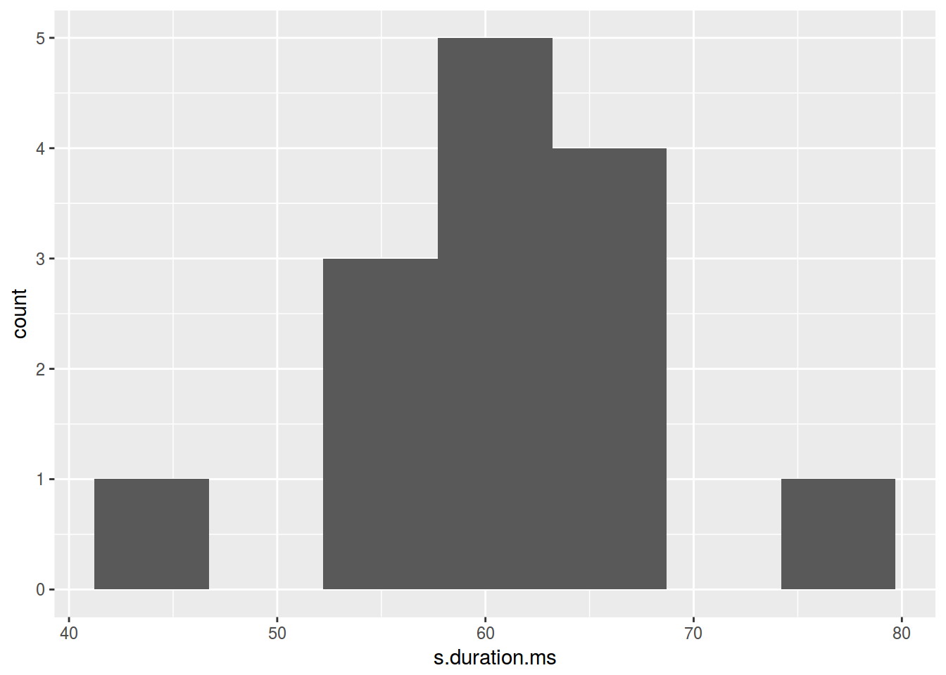
2.6.2 Гистограмма: цвет
ggplot(data = homo, aes(s.duration.ms)) +
  geom_histogram(fill = "lightblue")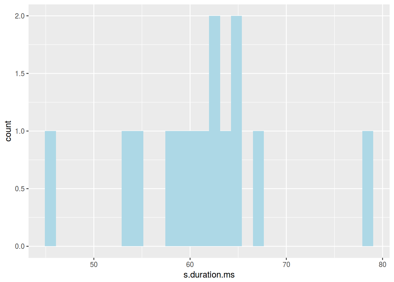
2.7.1 График плотности
ggplot(data = homo, aes(s.duration.ms)) +
  geom_density()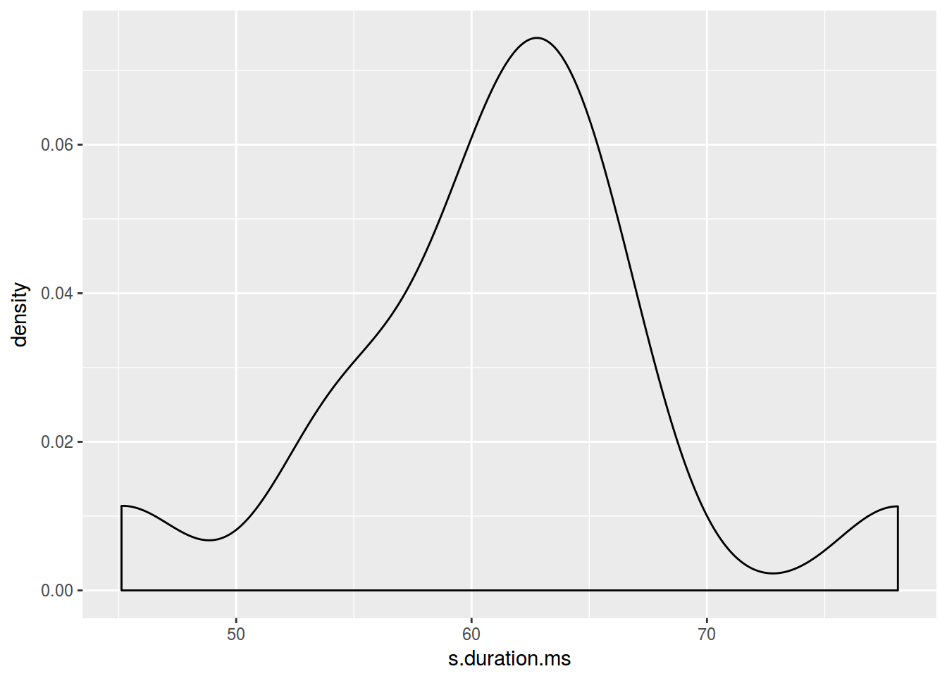
2.7.2 График плотности: цвет
ggplot(data = homo, aes(s.duration.ms)) +
  geom_density(fill = "lightblue")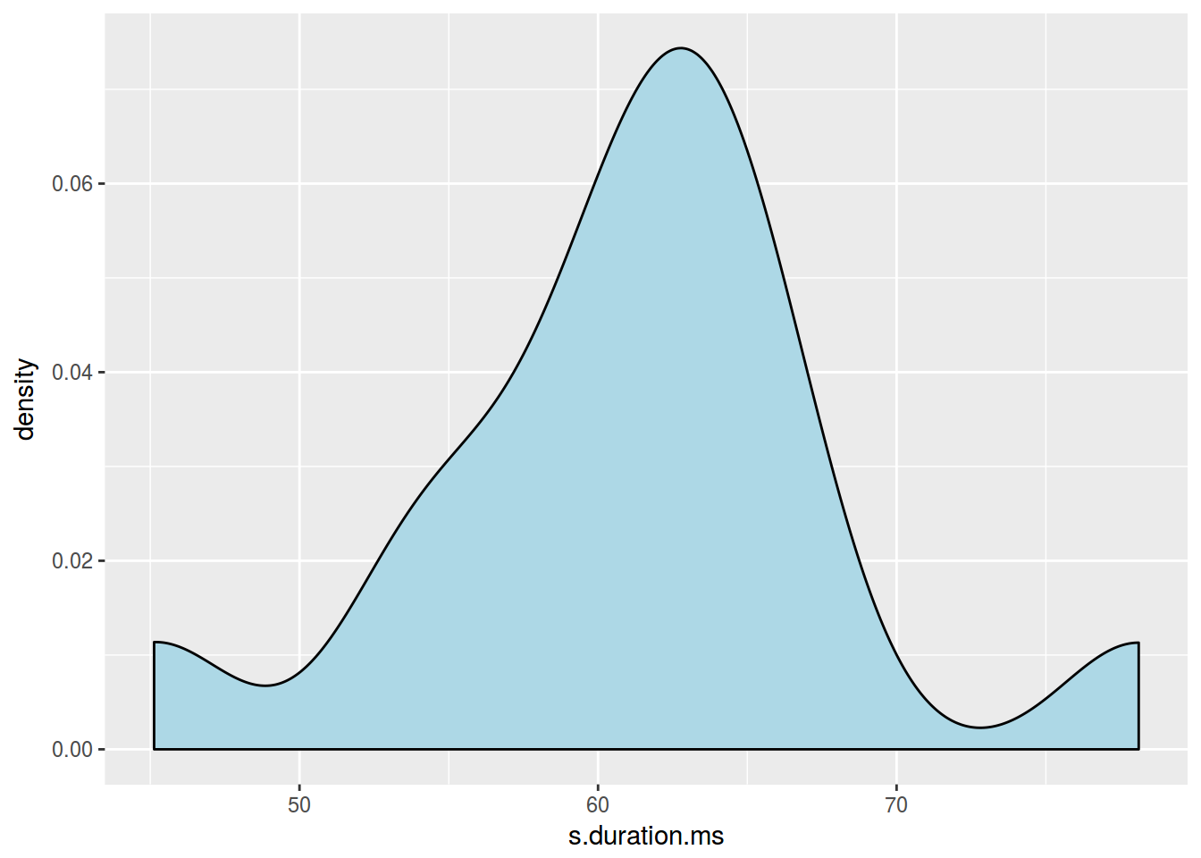
2.7.3 График плотности: несколько графиков
ggplot(data = homo, aes(s.duration.ms, fill = orientation)) +
  geom_density()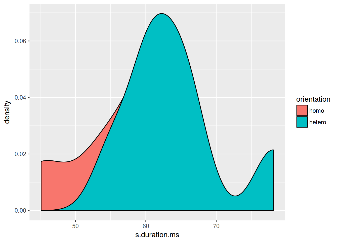
ggplot(data = homo, aes(s.duration.ms, fill = orientation)) +
  geom_density(alpha = 0.2)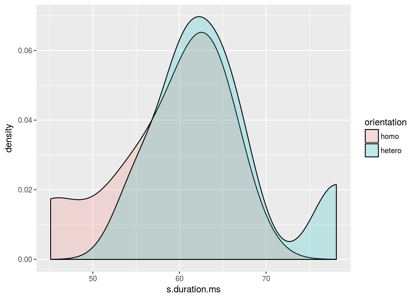
2.7.4 Joy plot
library(ggjoy)
ggplot(data = homo, aes(s.duration.ms, orientation)) +
  geom_joy()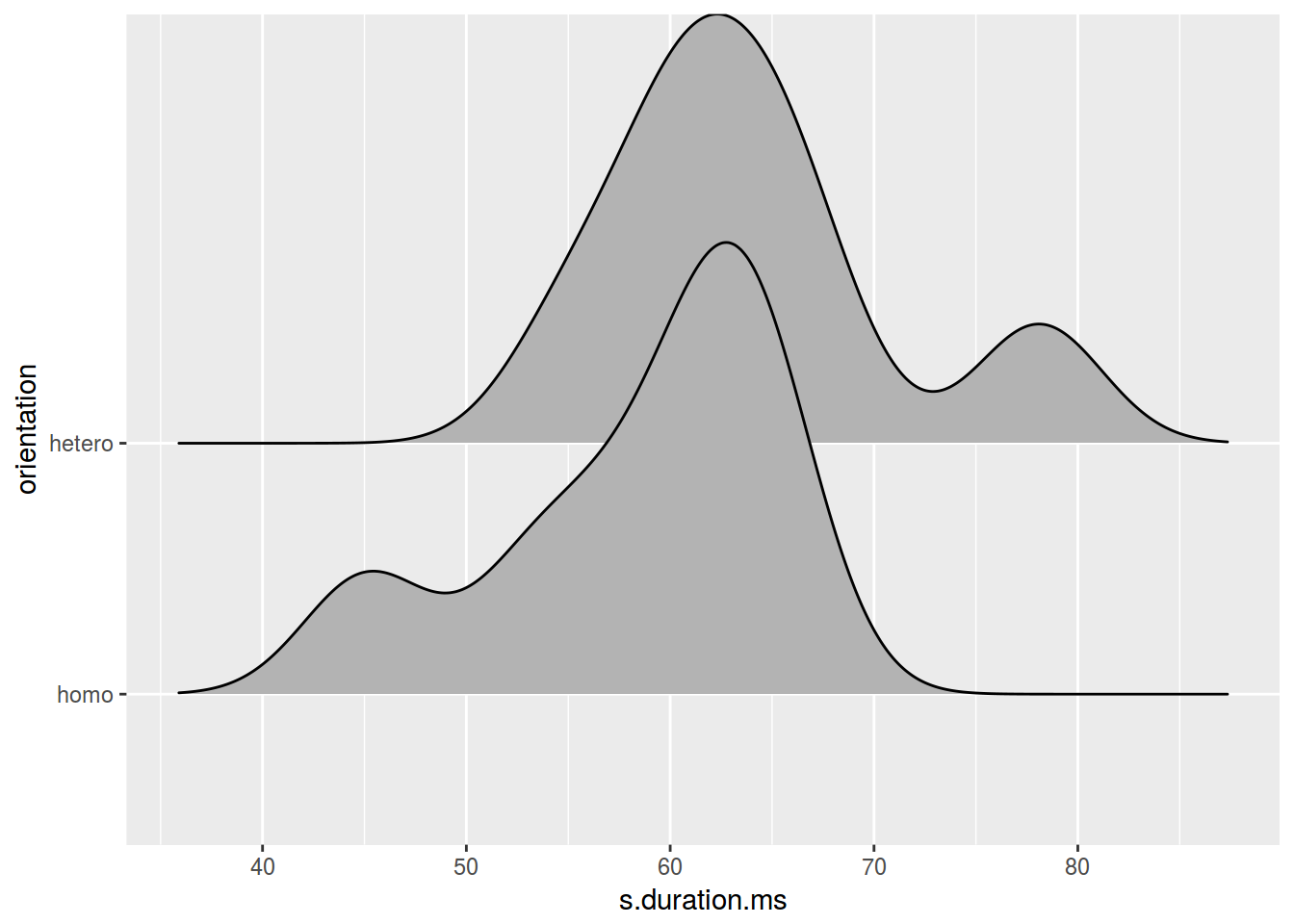
ggplot(data = homo, aes(s.duration.ms, orientation, fill = orientation)) +
  geom_joy()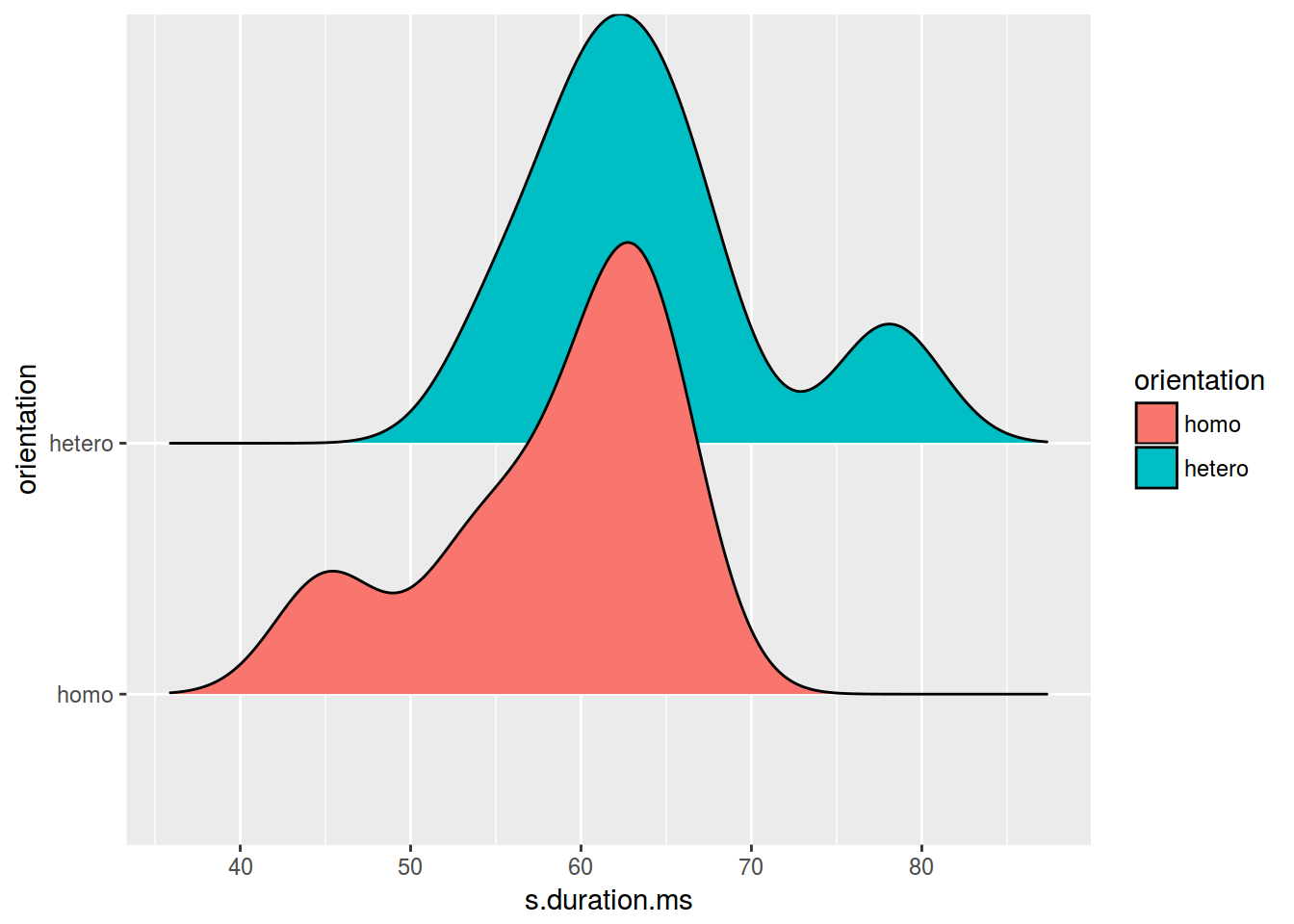
2.8.1 Facets: facet_wrap()
ggplot(data = homo, aes(speaker, s.duration.ms))+
  geom_point() +
  facet_wrap(~orientation)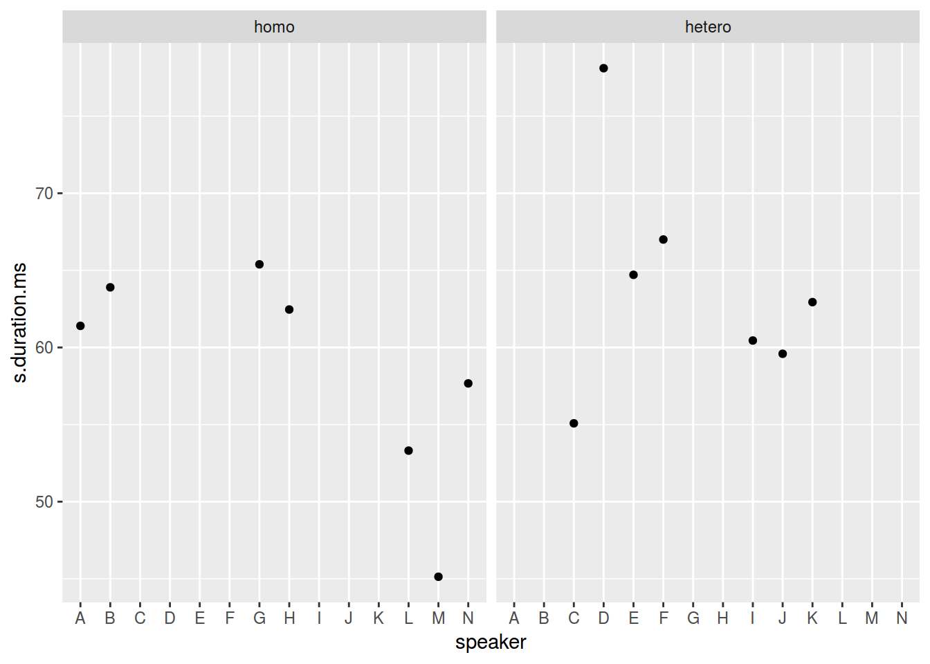
ggplot(data = homo, aes(speaker, s.duration.ms))+
  geom_point() +
  facet_wrap(~orientation, scales = "free")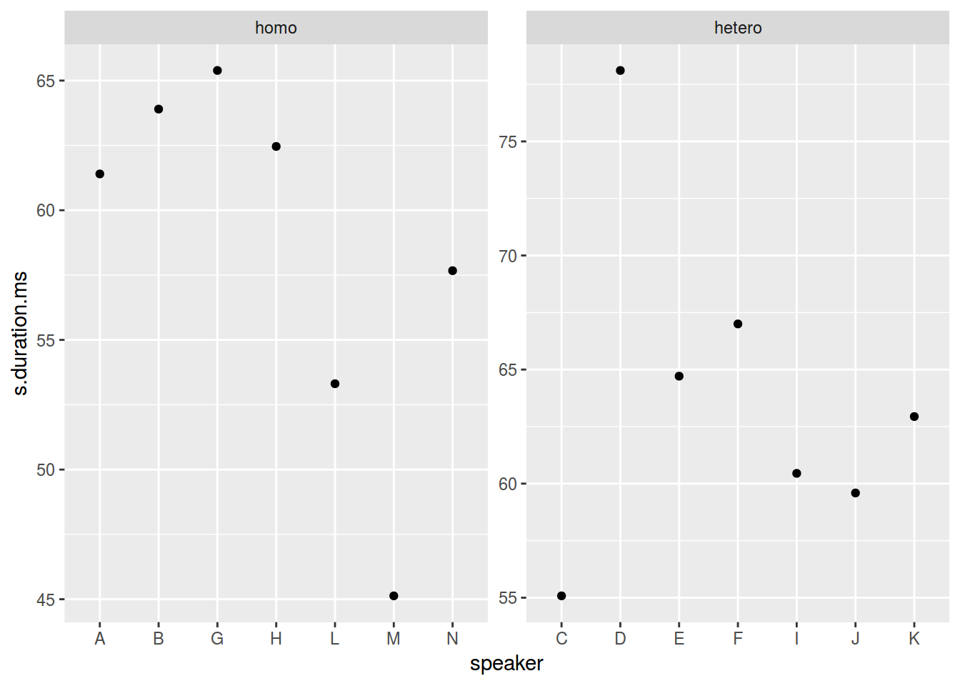
ggplot(data = homo, aes(speaker, s.duration.ms))+
  geom_point() +
  facet_wrap(~orientation, scales = "free_x")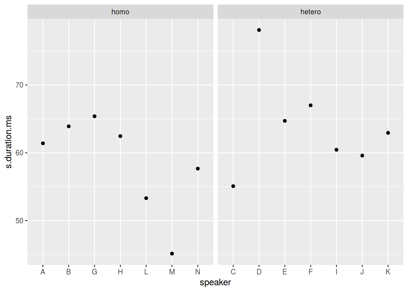
2.8.2 Facets: facet_grid()
homo$older_then_28 <- ifelse(homo$age > 28, "older", "younger")
ggplot(data = homo, aes(speaker, s.duration.ms))+
  geom_point() +
  facet_wrap(older_then_28~orientation, scales = "free_x")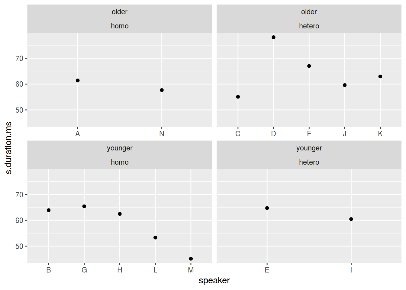
ggplot(data = homo, aes(speaker, s.duration.ms))+
  geom_point() +
  facet_grid(older_then_28~orientation, scales = "free_x")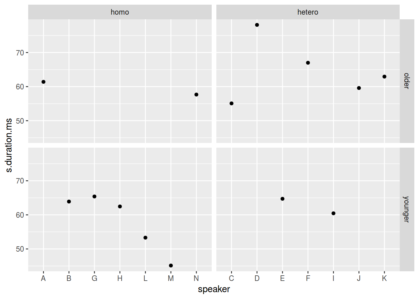
ggplot(data = homo, aes(speaker, s.duration.ms))+
  geom_point() +
  facet_grid(older_then_28~orientation, scales = "free_x", margins = TRUE)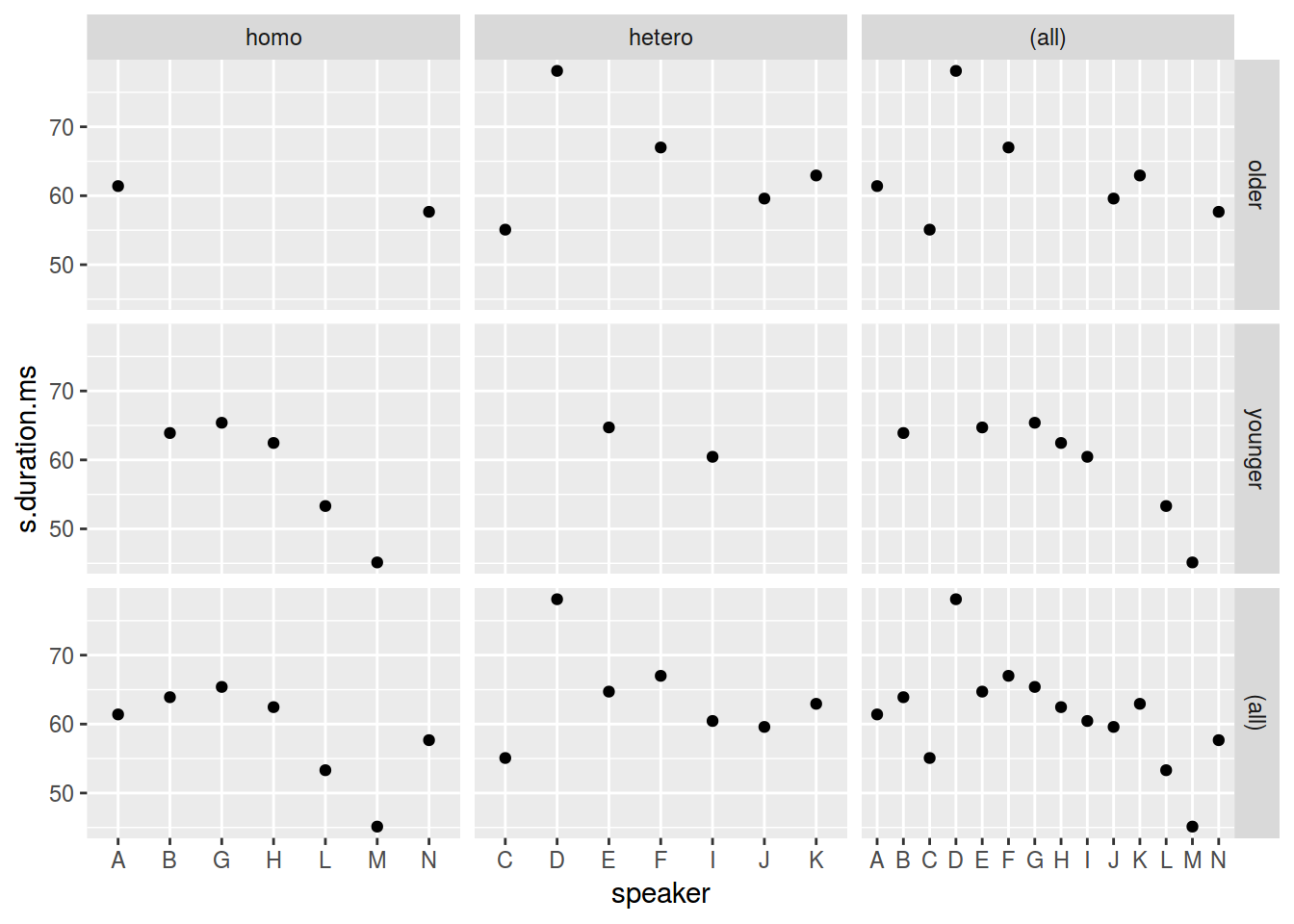
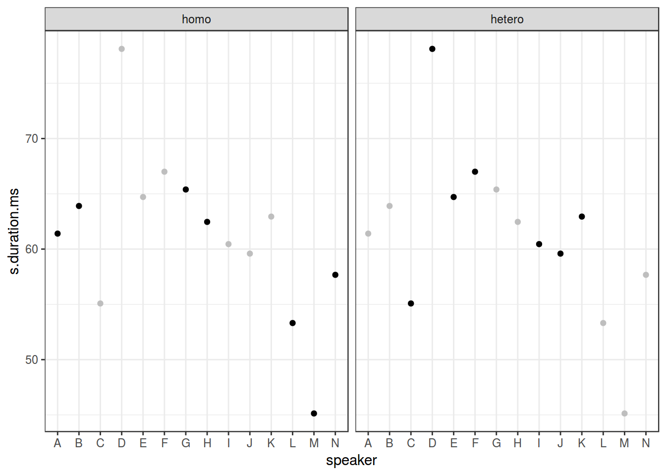
ggplot(data = homo, aes(speaker, s.duration.ms))+
  # Можно добавить geom без групирующей переменной!
  geom_point(data = homo[,-9], aes(speaker, s.duration.ms), color = "grey") +
  geom_point() +
  facet_wrap(~orientation)+
  theme_bw()