Lab 6.

0. Data

library(tidyverse)
np_acquisition <- read_csv("https://goo.gl/DhpmLe")
bnc_pron <- read_csv("https://goo.gl/vt1HCc")

1.1

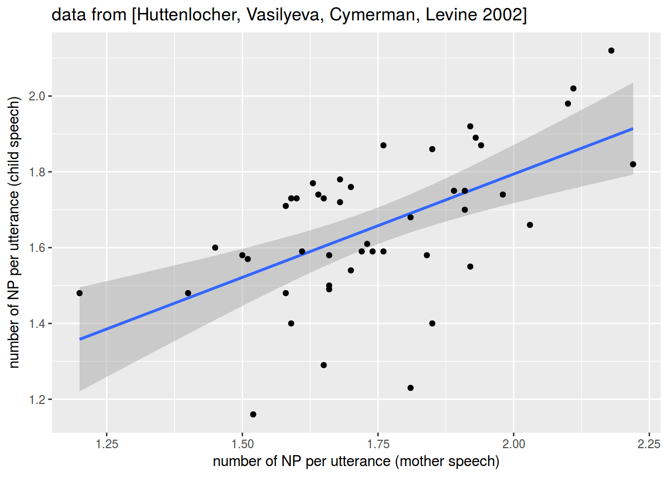
np_acquisition %>% 
  ggplot(aes(mother, child))+
  geom_smooth(method = "lm")+
  geom_point()+
  labs(x = "number of NP per utterance (mother speech)",
       y = "number of NP per utterance (child speech)",
       title = "data from [Huttenlocher, Vasilyeva, Cymerman, Levine 2002]")

1.2

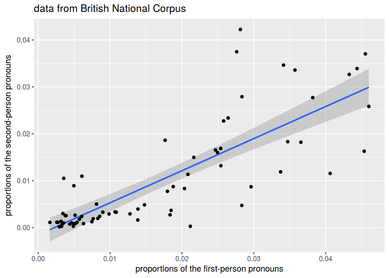
bnc_pron %>% 
  ggplot(aes(P1, P2))+
  geom_smooth(method = "lm")+
  geom_point()+
  labs(x = "proportions of the first-person pronouns",
       y = "proportions of the second-person pronouns",
       title = "data from British National Corpus")

2.1

# base R
cor(np_acquisition$child, np_acquisition$mother)

## [1] 0.5761599

# tidyverse
np_acquisition %>% 
  summarise(cor = cor(child, mother))

2.2

# base R
cor(bnc_pron$P1, bnc_pron$P2)

## [1] 0.8028283

# tidyverse
bnc_pron %>% 
  summarise(cor = cor(P1, P2))

3.1, 4.1

acq_fit <- lm(child ~ mother, data = np_acquisition)
summary(acq_fit)

## 
## Call:
## lm(formula = child ~ mother, data = np_acquisition)
## 
## Residuals:
##      Min       1Q   Median       3Q      Max 
## -0.46058 -0.08925  0.01071  0.13333  0.22770 
## 
## Coefficients:
##             Estimate Std. Error t value Pr(>|t|)    
## (Intercept)   0.7038     0.2051   3.432  0.00132 ** 
## mother        0.5452     0.1166   4.676 2.79e-05 ***
## ---
## Signif. codes:  0 '***' 0.001 '**' 0.01 '*' 0.05 '.' 0.1 ' ' 1
## 
## Residual standard error: 0.1627 on 44 degrees of freedom
## Multiple R-squared:  0.332,  Adjusted R-squared:  0.3168 
## F-statistic: 21.86 on 1 and 44 DF,  p-value: 2.789e-05

3.2, 4.2

bnc_fit <- lm(P1 ~ P2, data = bnc_pron)
summary(bnc_fit)

## 
## Call:
## lm(formula = P1 ~ P2, data = bnc_pron)
## 
## Residuals:
##       Min        1Q    Median        3Q       Max 
## -0.019234 -0.004895 -0.001672  0.003127  0.022450 
## 
## Coefficients:
##             Estimate Std. Error t value Pr(>|t|)    
## (Intercept) 0.007549   0.001307   5.778 2.15e-07 ***
## P2          0.942857   0.085543  11.022  < 2e-16 ***
## ---
## Signif. codes:  0 '***' 0.001 '**' 0.01 '*' 0.05 '.' 0.1 ' ' 1
## 
## Residual standard error: 0.008067 on 67 degrees of freedom
## Multiple R-squared:  0.6445, Adjusted R-squared:  0.6392 
## F-statistic: 121.5 on 1 and 67 DF,  p-value: < 2.2e-16

5.1

predict(acq_fit, newdata = data.frame(mother = 2))

##        1 
## 1.794163

5.2

predict(bnc_fit, newdata = data.frame(P2 = 0.04))

##         1 
## 0.0452634

6.1

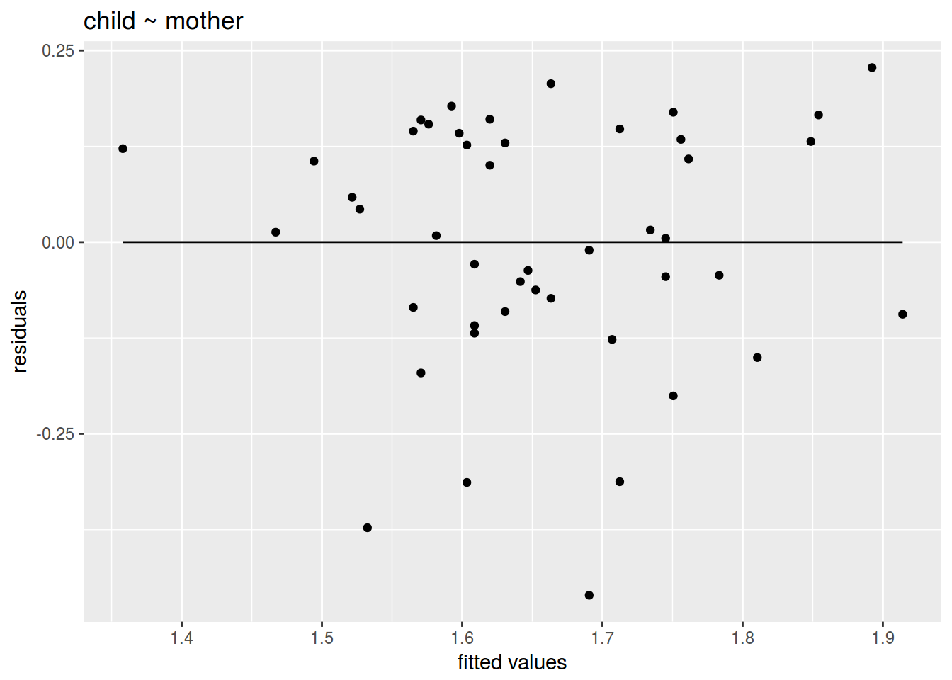
ggplot(data = acq_fit, aes(x = acq_fit$fitted.values, y = acq_fit$residuals))+
  geom_point()+
  geom_line(aes(y = 0))+
  labs(title = "child ~ mother",
       x = "fitted values",
       y = "residuals")

6.2

ggplot(data = bnc_fit, aes(x = bnc_fit$fitted.values, y = bnc_fit$residuals))+
  geom_point()+
  geom_line(aes(y = 0))+
  labs(title = "P1 ~ P2",
       x = "fitted values",
       y = "residuals")