Lab_15

library(tidyverse)
chekhov <- read_tsv("https://goo.gl/o18uj7")
chekhov %>% 
  mutate(trunc_titles = str_trunc(titles, 25, side = "right"),
         average = n/n_words) ->
  chekhov
head(chekhov)

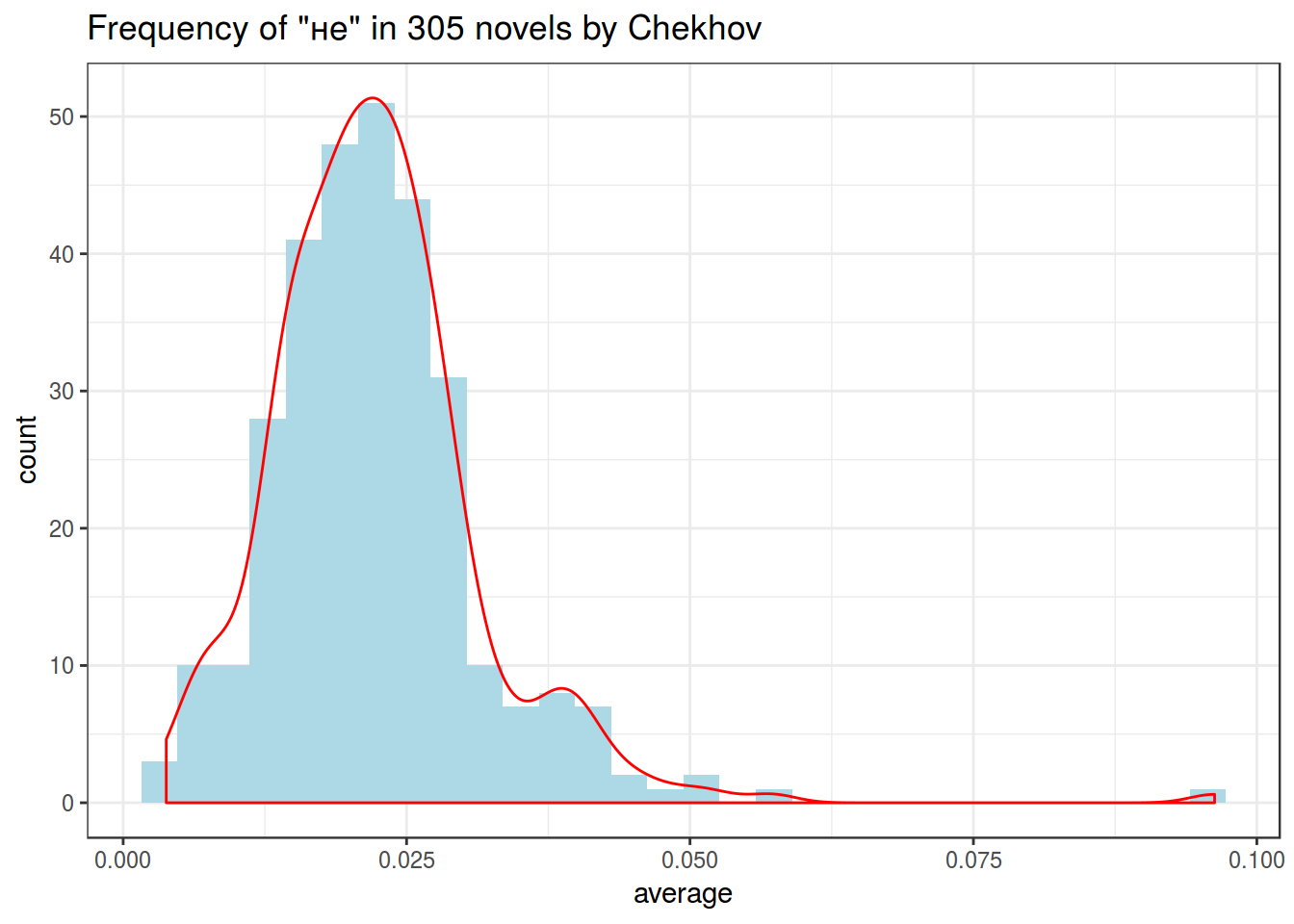
chekhov %>% 
  filter(word == "не") %>% 
  select(trunc_titles, word, average) %>% 
  ggplot(aes(average)) +
  geom_histogram(fill = "lightblue")+
  geom_density(color = "red")+
  theme_bw()+
  labs(title = 'Frequency of "не" in 305 novels by Chekhov')

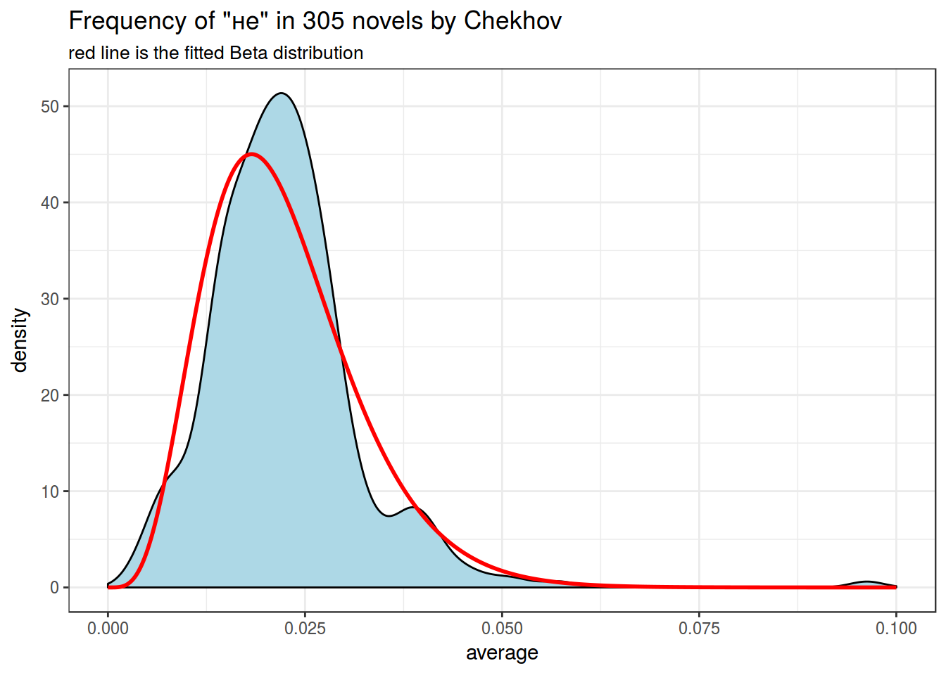
mu <- mean(chekhov$average[chekhov$word == "не"])
var <- var(chekhov$average[chekhov$word == "не"])
alpha0 <- ((1 - mu) / var - 1 / mu) * mu ^ 2
beta0 <- alpha0 * (1 / mu - 1)

x <- seq(0, 0.1, length = 1000)
estimation <- data_frame(
  x = x,
  density = c(dbeta(x, shape1 = alpha0, shape2 = beta0)))

chekhov %>% 
  filter(word == "не") %>% 
  select(trunc_titles, word, average) %>% 
  ggplot(aes(average)) +
  geom_density(fill = "lightblue")+
  geom_line(data = estimation, aes(x, density), color = "red", size = 1)+
  theme_bw()+
  labs(title = 'Frequency of "не" in 305 novels by Chekhov',
       subtitle = "red line is the fitted Beta distribution")

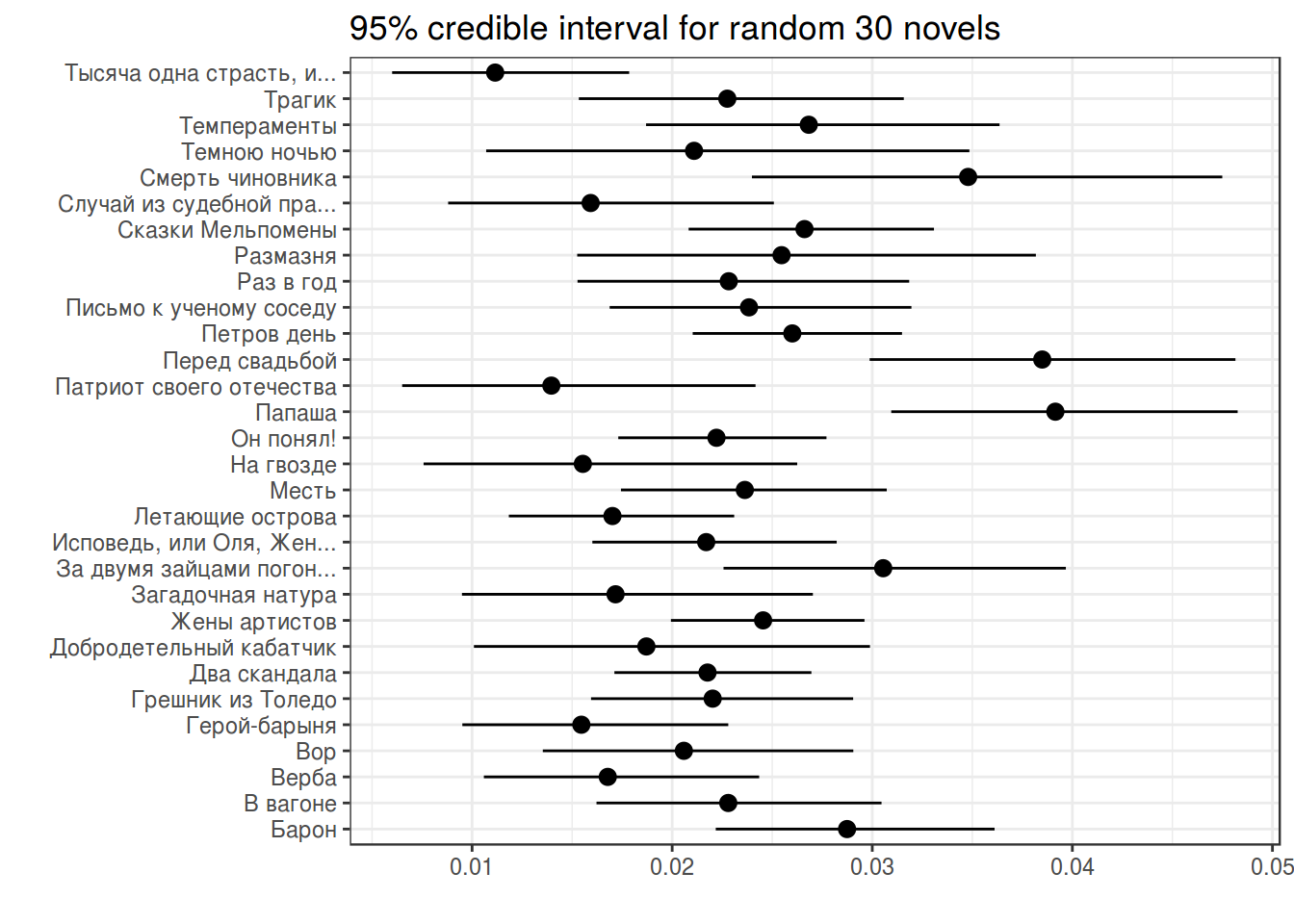
chekhov %>% 
  filter(word == "не") %>%
  slice(1:30) %>% 
  group_by(titles) %>% 
  mutate(alpha_post = n+alpha0,
         beta_post = n_words-n+beta0,
         average_post = alpha_post/(alpha_post+beta_post),
         cred_int_l = qbeta(.025, alpha_post, beta_post),
         cred_int_h = qbeta(.975, alpha_post, beta_post)) ->
  posterior

posterior %>% 
  select(titles, n_words, average, average_post) %>% 
  arrange(n_words)

posterior %>% 
  ggplot(aes(trunc_titles, average_post, ymin = cred_int_l, ymax = cred_int_h))+
  geom_pointrange()+
  coord_flip()+
  theme_bw()+
  labs(x = "", y = "", title = "95% credible interval for random 30 novels")