Lab 9. Linear mixed-effect models

Assignment link

library(tidyverse)
#install.packages("lingtypology")
library(lingtypology)
library(lme4)

1. Consonants and vowels

lapsyd <- read.csv("https://goo.gl/eD4S5n")
map.feature(lapsyd$name, features = lapsyd$area, 
              label = lapsyd$name,
              label.hide = TRUE)

fit1 <- lm(count_vowel~count_consonant, data = lapsyd)
summary(fit1)

## 
## Call:
## lm(formula = count_vowel ~ count_consonant, data = lapsyd)
## 
## Residuals:
##    Min     1Q Median     3Q    Max 
## -6.252 -2.992 -1.195  2.201 19.520 
## 
## Coefficients:
##                 Estimate Std. Error t value Pr(>|t|)    
## (Intercept)      7.38236    0.54784  13.475   <2e-16 ***
## count_consonant  0.04065    0.02274   1.787   0.0746 .  
## ---
## Signif. codes:  0 '***' 0.001 '**' 0.01 '*' 0.05 '.' 0.1 ' ' 1
## 
## Residual standard error: 4.093 on 400 degrees of freedom
## Multiple R-squared:  0.007923,   Adjusted R-squared:  0.005443 
## F-statistic: 3.195 on 1 and 400 DF,  p-value: 0.07464

lapsyd$model1 <- predict(fit1)

lapsyd %>% 
  ggplot(aes(count_consonant, count_vowel))+
  geom_point()+
  geom_line(aes(count_consonant, model1), color = "blue")+
  labs(x = "number of consonants",
       y = "number of vowels",
       caption = "data from LAPSyD")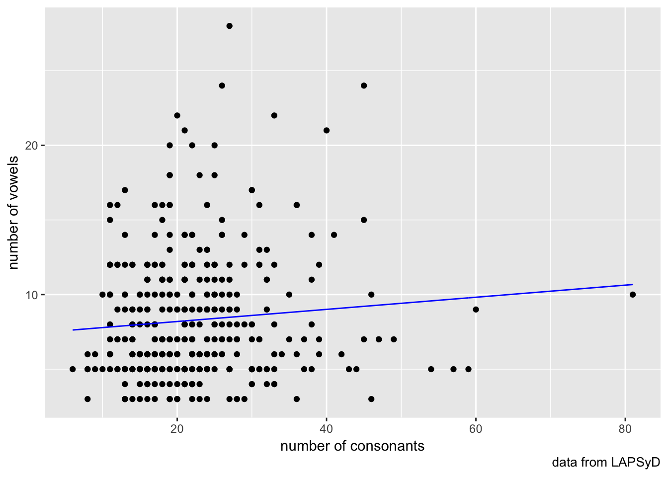

fit2 <- lmer(count_vowel ~ count_consonant + (1|area), data = lapsyd)
summary(fit2)

## Linear mixed model fit by REML ['lmerMod']
## Formula: count_vowel ~ count_consonant + (1 | area)
##    Data: lapsyd
## 
## REML criterion at convergence: 2242
## 
## Scaled residuals: 
##     Min      1Q  Median      3Q     Max 
## -1.5298 -0.6147 -0.2599  0.5146  4.7043 
## 
## Random effects:
##  Groups   Name        Variance Std.Dev.
##  area     (Intercept)  3.983   1.996   
##  Residual             14.753   3.841   
## Number of obs: 402, groups:  area, 6
## 
## Fixed effects:
##                 Estimate Std. Error t value
## (Intercept)       7.8928     0.9852   8.011
## count_consonant  -0.0111     0.0240  -0.463
## 
## Correlation of Fixed Effects:
##             (Intr)
## cont_cnsnnt -0.518

lapsyd$model2 <- predict(fit2)

lapsyd %>% 
  ggplot(aes(count_consonant, count_vowel))+
  geom_point()+
  geom_line(aes(count_consonant, model2, color = area))+
  labs(x = "number of consonants",
       y = "number of vowels",
       caption = "data from LAPSyD")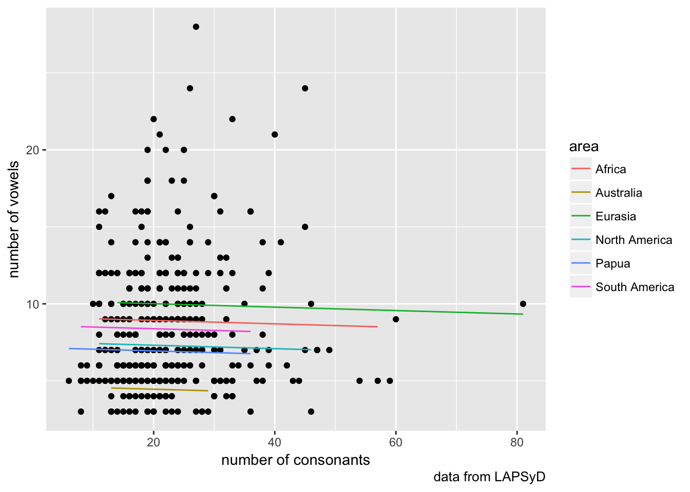

fit3 <- lmer(count_vowel ~ count_consonant + (1+count_consonant|area), data = lapsyd)
summary(fit3)

## Linear mixed model fit by REML ['lmerMod']
## Formula: count_vowel ~ count_consonant + (1 + count_consonant | area)
##    Data: lapsyd
## 
## REML criterion at convergence: 2236.4
## 
## Scaled residuals: 
##     Min      1Q  Median      3Q     Max 
## -1.7991 -0.6217 -0.2334  0.5299  4.7743 
## 
## Random effects:
##  Groups   Name            Variance Std.Dev. Corr 
##  area     (Intercept)     11.94558 3.4562        
##           count_consonant  0.01355 0.1164   -0.84
##  Residual                 14.32212 3.7845        
## Number of obs: 402, groups:  area, 6
## 
## Fixed effects:
##                  Estimate Std. Error t value
## (Intercept)      7.866281   1.555096   5.058
## count_consonant -0.005108   0.056987  -0.090
## 
## Correlation of Fixed Effects:
##             (Intr)
## cont_cnsnnt -0.854

lapsyd$model3 <- predict(fit3)

lapsyd %>% 
  ggplot(aes(count_consonant, count_vowel))+
  geom_point()+
  geom_line(aes(count_consonant, model3, color = area))+
  labs(x = "number of consonants",
       y = "number of vowels",
       caption = "data from LAPSyD")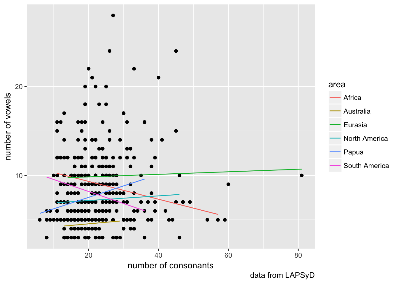

fit4 <- lmer(count_vowel ~ count_consonant + (0+count_consonant|area), data = lapsyd)
summary(fit4)

## Linear mixed model fit by REML ['lmerMod']
## Formula: count_vowel ~ count_consonant + (0 + count_consonant | area)
##    Data: lapsyd
## 
## REML criterion at convergence: 2250.8
## 
## Scaled residuals: 
##     Min      1Q  Median      3Q     Max 
## -1.5967 -0.6774 -0.2688  0.4497  4.6750 
## 
## Random effects:
##  Groups   Name            Variance  Std.Dev.
##  area     count_consonant  0.008151 0.09028 
##  Residual                 15.093094 3.88498 
## Number of obs: 402, groups:  area, 6
## 
## Fixed effects:
##                 Estimate Std. Error t value
## (Intercept)      8.68579    0.59439  14.613
## count_consonant -0.05519    0.04649  -1.187
## 
## Correlation of Fixed Effects:
##             (Intr)
## cont_cnsnnt -0.563

lapsyd$model4 <- predict(fit4)

lapsyd %>% 
  ggplot(aes(count_consonant, count_vowel))+
  geom_point()+
  geom_line(aes(count_consonant, model4, color = area))+
  labs(x = "number of consonants",
       y = "number of vowels",
       caption = "data from LAPSyD")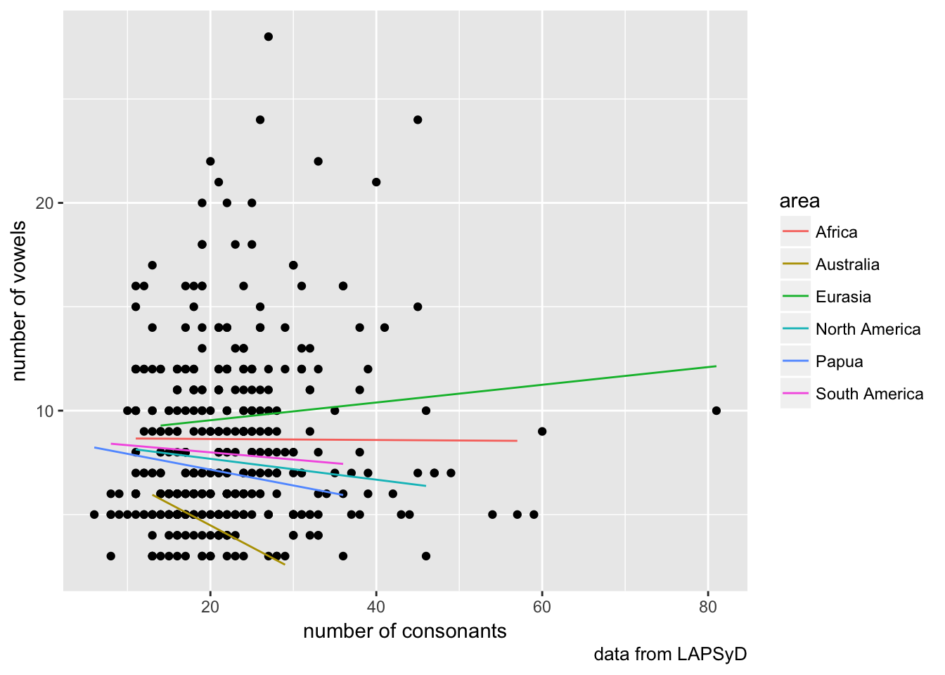

fit5 <- lmer(count_vowel ~ count_consonant + (1|area) + (0+count_consonant|area), data = lapsyd)
summary(fit5)

## Linear mixed model fit by REML ['lmerMod']
## Formula: 
## count_vowel ~ count_consonant + (1 | area) + (0 + count_consonant |  
##     area)
##    Data: lapsyd
## 
## REML criterion at convergence: 2239.8
## 
## Scaled residuals: 
##     Min      1Q  Median      3Q     Max 
## -1.6499 -0.6023 -0.2494  0.5018  4.7428 
## 
## Random effects:
##  Groups   Name            Variance Std.Dev.
##  area     (Intercept)      5.67146 2.38148 
##  area.1   count_consonant  0.00606 0.07785 
##  Residual                 14.42645 3.79822 
## Number of obs: 402, groups:  area, 6
## 
## Fixed effects:
##                 Estimate Std. Error t value
## (Intercept)      8.19243    1.15107   7.117
## count_consonant -0.02700    0.04326  -0.624
## 
## Correlation of Fixed Effects:
##             (Intr)
## cont_cnsnnt -0.337

lapsyd$model5 <- predict(fit5)

lapsyd %>% 
  ggplot(aes(count_consonant, count_vowel))+
  geom_point()+
  geom_line(aes(count_consonant, model5, color = area))+
  labs(x = "number of consonants",
       y = "number of vowels",
       caption = "data from LAPSyD")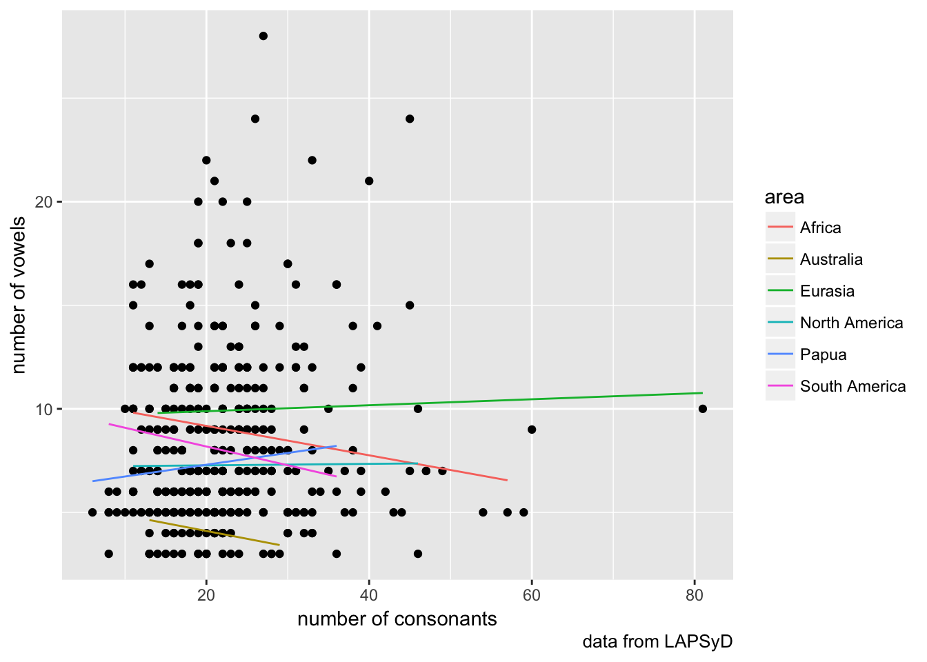

anova(fit5, fit4, fit3, fit2, fit1)

## refitting model(s) with ML (instead of REML)

2. Icelandic vowels

This set is based on (Coretta 2017, https://goo.gl/NrfgJm). This dissertation deals with the relation between vowel duration and aspiration in consonants. Author carried out a data collection with 5 natives speakers of Icelandic. Then he extracted the duration of vowels followed by aspirated versus non-aspirated consonants. Check out whether the vowels before consonants of different places of articulation are significantly different.

Use read.csv(“https://goo.gl/7gIjvK”) for downloading data.

2.1

Calculate mean values for vowel duration in your data grouped by place (of articulation) and speaker.

df <- read.csv("https://goo.gl/7gIjvK")

df %>% 
  group_by(place, speaker) %>% 
  summarise(mean(vowel.dur))

Let’s do some visualization

df %>% 
  ggplot(aes(place, vowel.dur)) + 
    geom_point(alpha = 0.2) + 
    facet_wrap(~ speaker) + 
    xlab("place of articulation") + 
    ylab("vowel duration")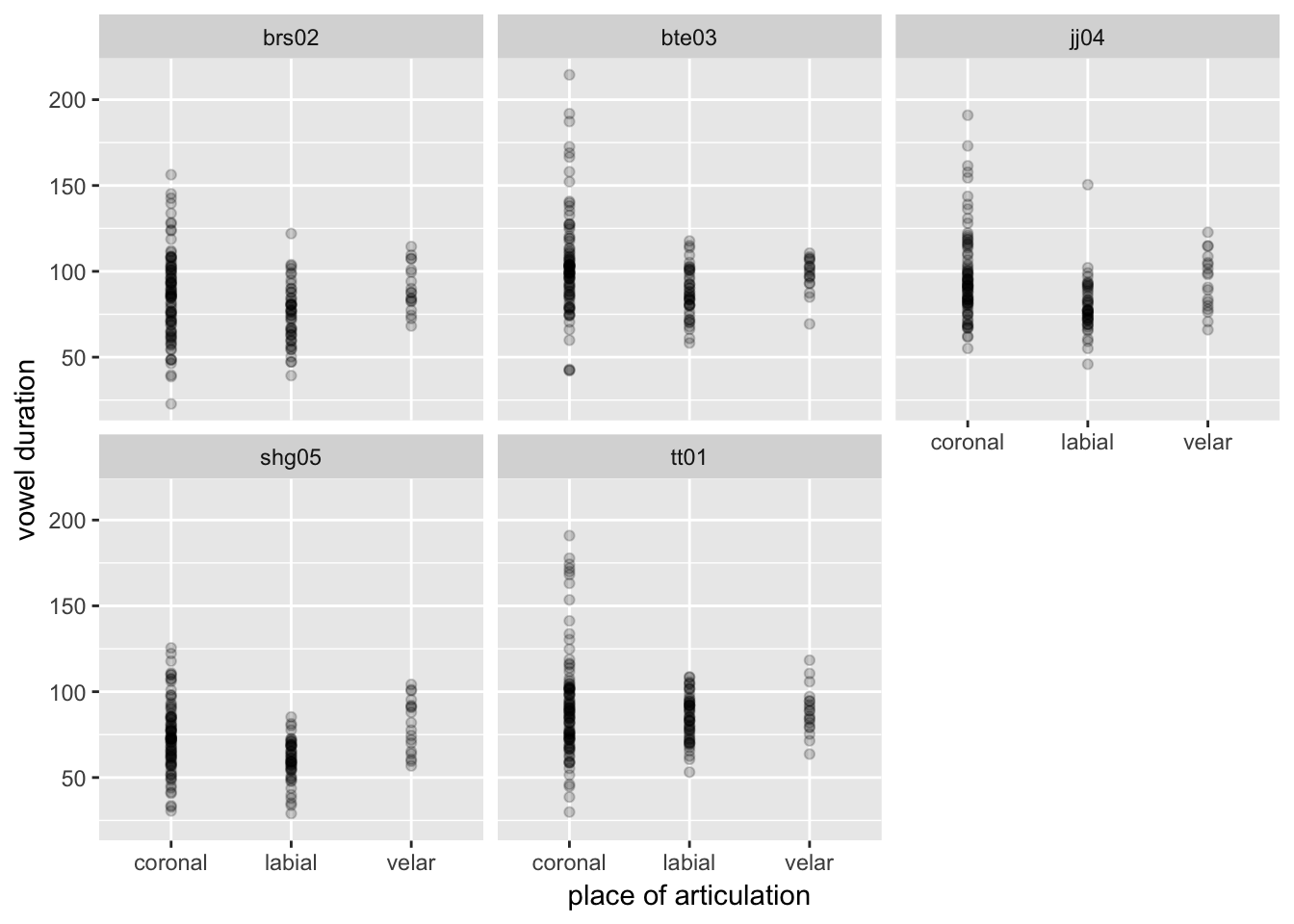

2.2 Calculate mean values for vowel duration in your data grouped by `word`.

df <- read.csv("https://goo.gl/7gIjvK")

df %>% 
  group_by(word) %>% 
  summarise(mean(vowel.dur))

2.3 Fit mixed-effect linear regression model

taking into account speaker as a random effect. Plot

fit <- lmer(vowel.dur ~ place + (1|speaker), data = df)
summary(fit)

## Linear mixed model fit by REML ['lmerMod']
## Formula: vowel.dur ~ place + (1 | speaker)
##    Data: df
## 
## REML criterion at convergence: 7292.9
## 
## Scaled residuals: 
##     Min      1Q  Median      3Q     Max 
## -2.9226 -0.5708 -0.0926  0.4450  5.0208 
## 
## Random effects:
##  Groups   Name        Variance Std.Dev.
##  speaker  (Intercept) 111.6    10.57   
##  Residual             495.8    22.27   
## Number of obs: 806, groups:  speaker, 5
## 
## Fixed effects:
##             Estimate Std. Error t value
## (Intercept)  90.9320     4.8361  18.803
## placelabial -13.3303     1.7503  -7.616
## placevelar   -0.7663     2.5516  -0.300
## 
## Correlation of Fixed Effects:
##             (Intr) plclbl
## placelabial -0.126       
## placevelar  -0.086  0.238

plot(fit)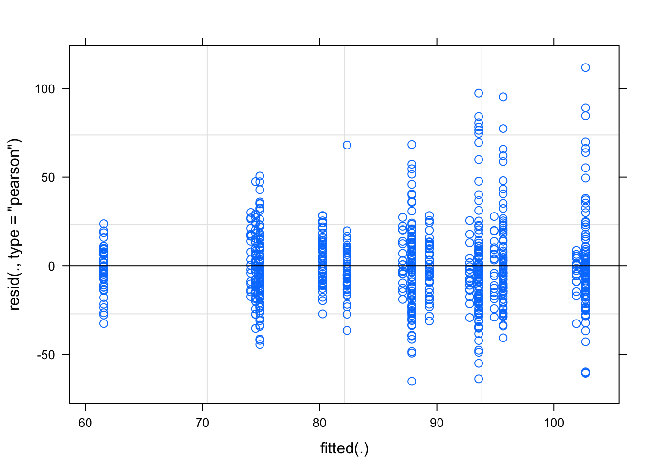

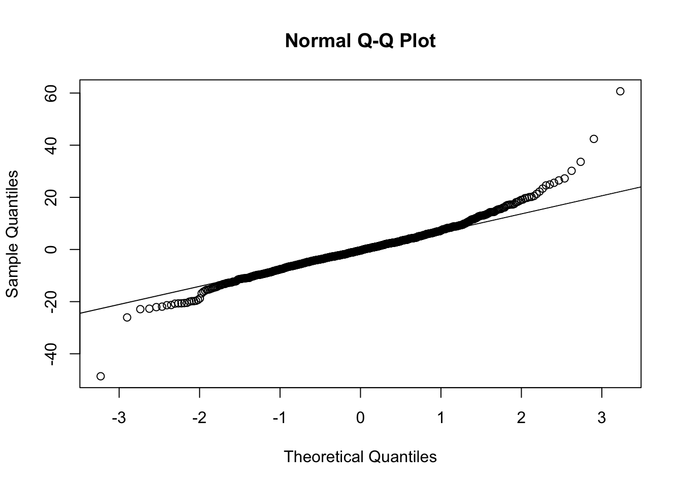
qqnorm(resid(fit))
qqline(resid(fit))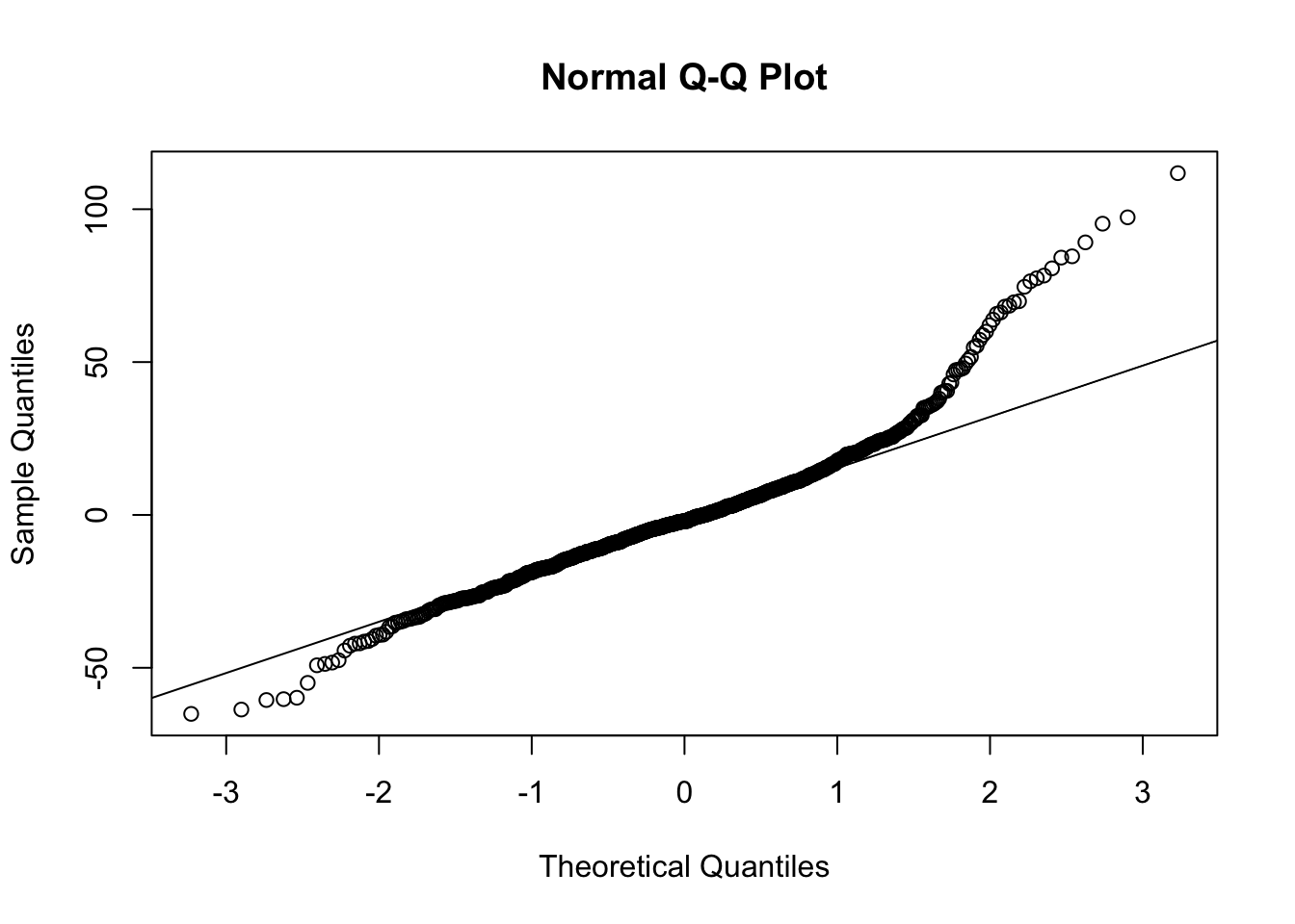

2.3 Fit mixed-effect linear regression model

taking into account speaker and word as random effects. Note that random factors can be nested.

If our groups are nested (as it happens with speakers and words), the following model should be wrong:

fit2.WRONG <- lmer(vowel.dur ~ place + (1|speaker) + (1|word), data = df)  # treats the two random effects as if they are crossed

To avoid future confusion let us create a new variable that is explicitly nested. Let???s call it sample:

df <- within(df, sample <- factor(speaker:word))
head(summary(df$sample))

## bte03:d\303\266gg  tt01:d\303\266gg        tt01:kampa       brs02:detta 
##                 6                 4                 4                 3 
##        brs02:duld        brs02:dult 
##                 3                 3

Now let’s fit the nested mixed-effect model properly:

fit2 <- lmer(vowel.dur ~ place + (1|speaker) + (1|sample), data = df)  # treats the two random effects as if they are nested
summary(fit2)

## Linear mixed model fit by REML ['lmerMod']
## Formula: vowel.dur ~ place + (1 | speaker) + (1 | sample)
##    Data: df
## 
## REML criterion at convergence: 6745.1
## 
## Scaled residuals: 
##     Min      1Q  Median      3Q     Max 
## -4.6053 -0.4657 -0.0336  0.4225  5.7479 
## 
## Random effects:
##  Groups   Name        Variance Std.Dev.
##  sample   (Intercept) 390.9    19.77   
##  speaker  (Intercept) 105.6    10.28   
##  Residual             111.5    10.56   
## Number of obs: 806, groups:  sample, 273; speaker, 5
## 
## Fixed effects:
##             Estimate Std. Error t value
## (Intercept)  91.0944     4.8795  18.669
## placelabial -13.4685     2.7927  -4.823
## placevelar   -0.9022     4.1740  -0.216
## 
## Correlation of Fixed Effects:
##             (Intr) plclbl
## placelabial -0.197       
## placevelar  -0.132  0.231

plot(fit2)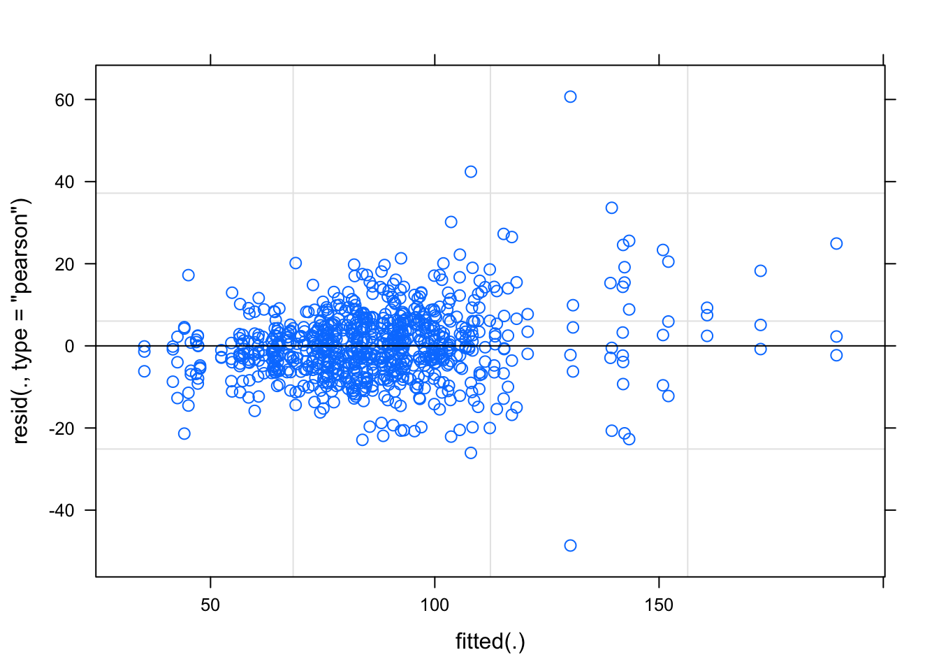

qqnorm(resid(fit2))
qqline(resid(fit2))

Lab 9. Linear mixed-effect models

Assignment link

1. Consonants and vowels

2. Icelandic vowels

2.1

2.2 Calculate mean values for vowel duration in your data grouped by word.

2.3 Fit mixed-effect linear regression model

2.3 Fit mixed-effect linear regression model

2.2 Calculate mean values for vowel duration in your data grouped by `word`.