- Empirical Bayes Estimation
O. Lyashevskaya, G. Moroz, I. Schurov
1. Probability destribution
- A probability value must be nonnegative.
- The sum of the probabilities across all events in the entire sample space must be 1.
- For any two mutually exclusive events, the probability that one or the other occurs is the sum of their individual probabilities.
Discrete case:
\[p(⚀) + p(⚁) + p(⚂) + p(⚃) + p(⚄) + p(⚅) = \sum_{i = 0}^{n} p(x_i) = 1\]
Continuouse case:
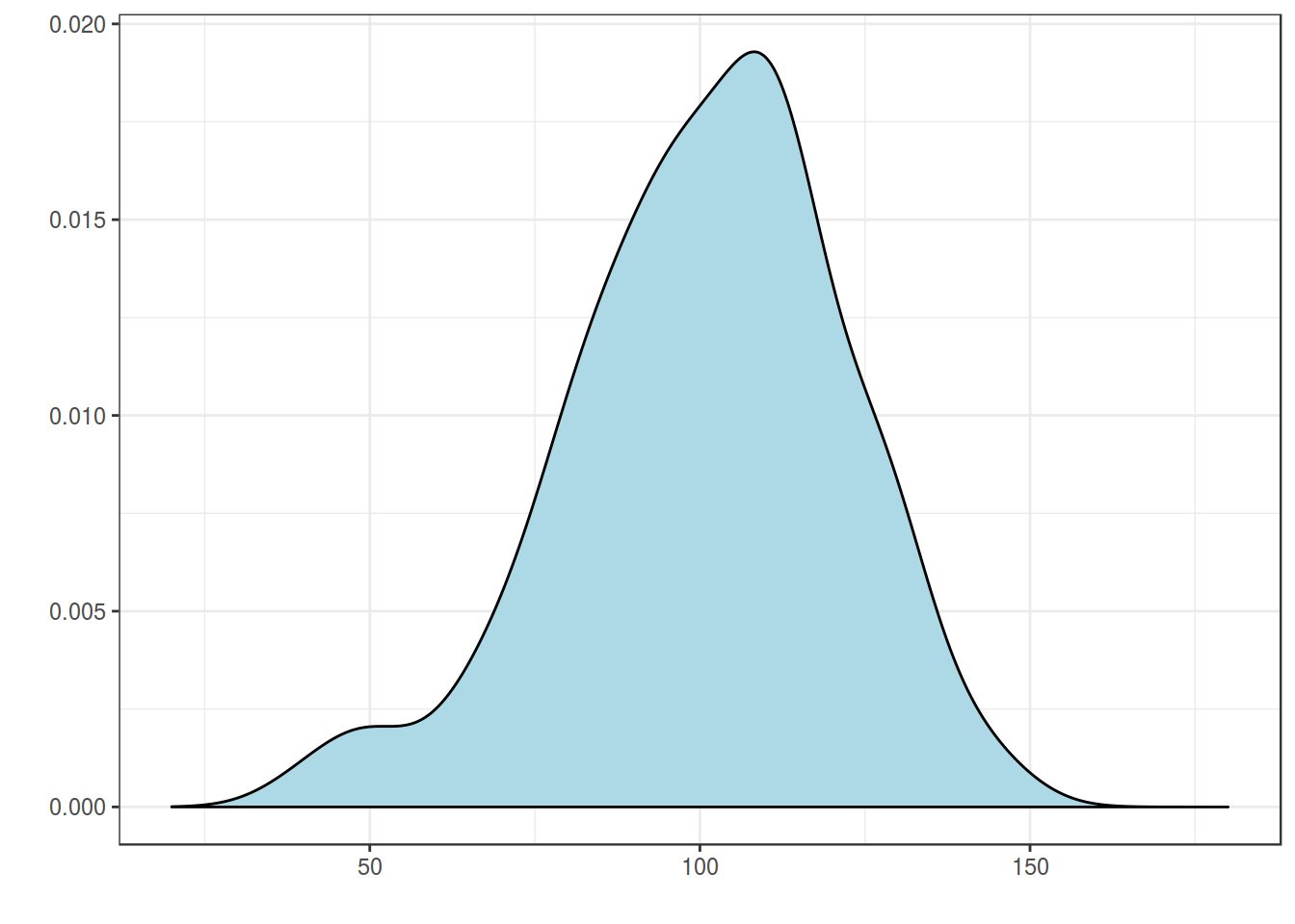 \[ = \int p(x)dx = 1\]
2. Two-way destribution
Joint probability
\[p(A, B) = p(B, A)\]
Conditional probability
\[p(B|A) = p(A, B)/P(A)\]
Discrete case:
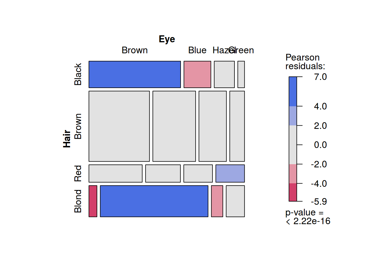
- joint probability: probability of having blue eyesand blond hair: \[p(Hair = Blond, Eye = Blue) = p(Eye = Blue, Hair = Blond) = 0.16\]
- conditional probability: probability of having blond hair, if eyes are blue: \[p(Hair = Blond|Eye = Blue) = \frac{p(Eye = Blue, Hair = Blond)}{\sum_{i=1}^{n} p(Eye = Blue, Hair = x_i)} = \frac{0.16}{0.36} \approx 0.45\]
Continuouse case:
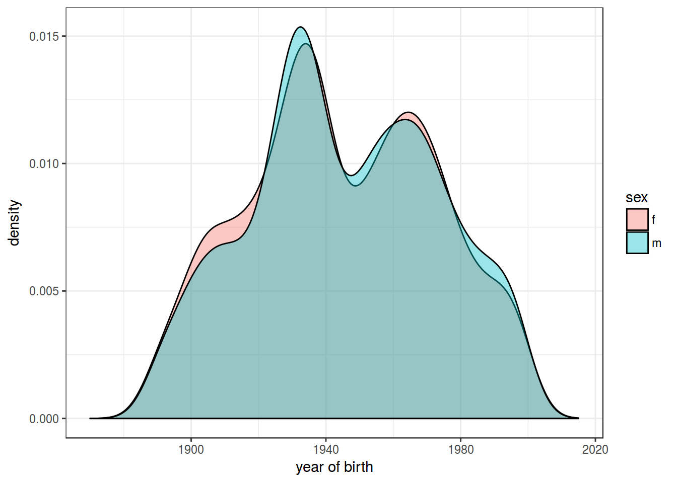
- joint probability: probability of having blue eyesand blond hair: \[p(sex = f, year = 1945) = p(year = 1945, sex = f)\]
- conditional probability: probability of having blond hair, if eyes are blue: \[p(year = 1945|sex = f) = \frac{p(sex = f, year = 1945)}{\int p(sex = f, year = x)dx}\]
3. Bayes rule
\[p(A|B) = \frac{p(A, B)}{p(B)}\Rightarrow p(A|B) \times p(B) = p(A, B)\] \[p(B|A) = \frac{p(B, A)}{p(A)}\Rightarrow p(B|A) \times p(A) = p(B, A)\] \[p(A|B) \times p(B) = p(B|A) \times p(A)\] \[p(A|B) = \frac{p(B|A)p(A)}{p(B)}\]
Discrete case:
\[p(A|B) = \frac{p(B|A)p(A)}{\sum_{i=1}^{n} p(B, a_i) \times p(a_i)}\]
Continuouse case:
\[p(A|B) = \frac{p(B|A)p(A)}{\int p(B, a) \times p(a)da}\]
what is happening in numerator:
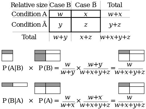
what is happening during the division:
\[\frac{w}{w+x+y+z}:\frac{w+x}{w+x+y+z} = \frac{w}{w+x}\]
4. Bayes inference
- p(θ) — parametor values
- p(Data) — data values
\[p(θ|Data) = \frac{p(Data|θ)\times p(θ)}{p(Data)}\]
- p(θ|Data) — posterior
- p(Data|θ) — likelihood, conjugate prior
- p(θ) — prior
- p(Data) — data
Bayes’ rule gets us from a prior belief, p(θ), to a posterior belief, p(θ|D), when we take into account some data D. Now suppose we observe some more data, which we’ll denote D’. We can then update our beliefs again, from p(θ|D) to p(θ|D’, D). Does our final belief depend on whether we update with D first and D’ second, or update with D’ first and D second?
\[p(θ|Data, Data') = p(θ|Data', Data)\]
So for correct modeling we need to know destribution family and conjugate prior:
5. Binomial and Beta destributions
\[P(k | n, θ) = \frac{n!}{k!(n-k)!} \times θ^k \times (1-θ)^{n-k} = {n \choose k} \times θ^k \times (1-θ)^{n-k}\] \[ 0 \leq θ \leq 1; n, k > 0\]

\[P(x; α, β) = \frac{x^{α-1}\times (1-x)^{β-1}}{B(α, β)}; 0 \leq x \leq 1; α, β > 0\] Beta function: \[Β(α, β) = \frac{Γ(α)\times Γ(β)}{Γ(α+β)} = \frac{(α-1)!(β-1)!}{(α+β-1)!} \]
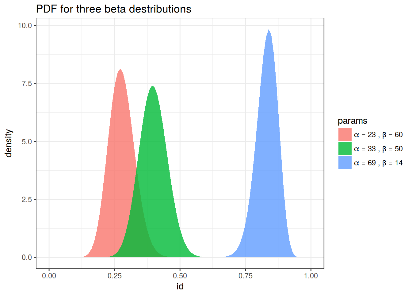
shiny::runGitHub("agricolamz/beta_distribution_shiny") 6. Binomial example
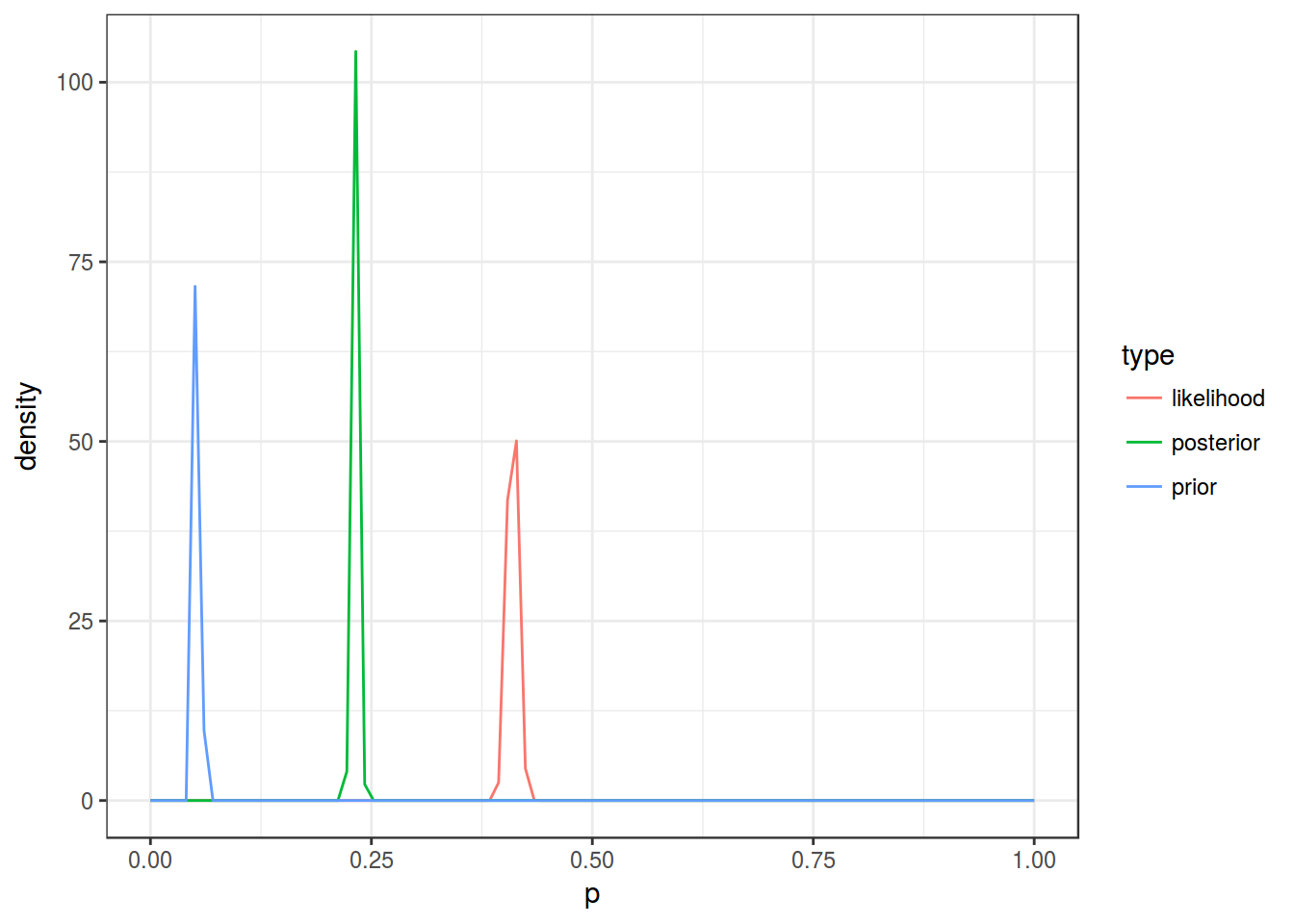
In corpus based frequency dictionary noun не has frequency 0.05389. In some text (61981 words) this preposition appears 2540 times. How does it change our prior knoledge?
- p(θ) — prior is a Beta destribution
- p(Data|θ) — conjugate prior is a Binomial destribution
- p(θ|Data) — posterior is a Beta destribution
p(Data) — … we don’t need it since numerator is Beta destribution
Alpha and beta for prior destribution \[\mu = \frac{\alpha}{\alpha+\beta} \Rightarrow \alpha = \mu \times (\alpha+\beta) = 6198 \times 0.05389 \approx 3330.156\] \[\beta = 6198 - 3340.156 = 2857.844\]
Alpha and beta for posterior destribution \[\alpha_{posterior} = \alpha_{prior} + \# success = 3340.156 + 2540 \] \[\beta_{posterior} = \beta_{prior} + \# failure = 2857.844 + 6198 - 2540\]
7. How stop be afraid of choosing a prior?
- Prior is the way of incorporating previous knowledge.
- Prior is more scintific way of thinking.
- If you are really scared you coud choose non-informative prior.
- … sometimes you have a trick — Empirical Bayes Estimation.
Empirical Bayes estimation
Then we could calculate proportion of “не” in each of them. After that it is possible to approximate a Beta destribution from the destribution of “не” proportions from different novels and use it as a prior. What we will get is a shrinked mean. The true outliers will be vissible then.
The easeast and the worst way to fit the Beta destribution. From this systme of equations:
\[\mu = \frac{\alpha}{\alpha+\beta}\] \[\sigma = \frac{\alpha\times\beta}{(\alpha+\beta)^2\times(\alpha+\beta+1)}\]
…we can get \(\alpha\) and \(\beta\):
\[\alpha = \left(\frac{1-\mu}{\sigma^2} - \frac{1}{\mu}\right)\times \mu^2\] \[\beta = \alpha\times\left(\frac{1}{\mu} - 1\right)\]
