- Basic Statistics
G. Moroz
library(tidyverse)1.1 Descriptive statistics
homo <- read_csv("http://goo.gl/Zjr9aF")
homo %>%
  summarise(mean = mean(s.duration.ms),
            trimed_mean = mean(s.duration.ms, trim = 0.2),
            weighted_mean = weighted.mean(s.duration.ms, age),
            median = median(s.duration.ms),
            min = min(s.duration.ms),
            max = max(s.duration.ms),
sd = sd(s.duration.ms))summary(homo)## speaker s.duration.ms vowel.duration.ms average.f0.Hz
## Length:14 Min. :45.13 Min. : 93.68 Min. :100.3
## Class :character 1st Qu.:58.15 1st Qu.:118.31 1st Qu.:116.0
## Mode :character Median :61.93 Median :123.75 Median :122.7
## Mean :61.22 Mean :124.06 Mean :125.2
## 3rd Qu.:64.51 3rd Qu.:132.27 3rd Qu.:130.3
## Max. :78.11 Max. :147.52 Max. :155.3
## f0.range.Hz perceived.as.homo perceived.as.hetero
## Min. : 37.40 Min. : 4.00 Min. : 4.00
## 1st Qu.: 53.30 1st Qu.: 8.25 1st Qu.: 5.00
## Median : 73.20 Median :12.50 Median :12.50
## Mean : 76.66 Mean :13.50 Mean :11.50
## 3rd Qu.:102.53 3rd Qu.:20.00 3rd Qu.:16.75
## Max. :118.20 Max. :21.00 Max. :21.00
## perceived.as.homo.percent orientation age
## Min. :0.16 Length:14 Min. :19.00
## 1st Qu.:0.33 Class :character 1st Qu.:22.75
## Median :0.50 Mode :character Median :28.50
## Mean :0.54 Mean :27.86
## 3rd Qu.:0.80 3rd Qu.:30.00
## Max. :0.84 Max. :40.001.2 Common words
Statistics are used much like a drunk uses a lamppost: for support, not illumination. A.E. Housman (commonly attributed to Andrew Lang)
- frequentist vs. bayesian statistics > A frequentist uses impeccable logic to answer the wrong question, while a Bayesean answers the right question by making assumptions that nobody can fully believe in. P. G. Hammer
test parameters:
- parametric vs. nonparametric tests
- one sample vs. two sample tests vs. multiple sample tests
- paired vs. not paired tests
- one-tailed vs. two-tailed tests
2. One sample test
2.1 Confident interval
\[\bar{x} \pm z \times \frac{\sigma}{\sqrt{n}}\]
Where is standard error?
z — z-score, for 95% CI it is 1.96, for 99% CI it is 2.58
homo %>%
  summarise(mean = mean(s.duration.ms),
            ci = 1.96 * sd(s.duration.ms)/sqrt(n()),
            min = mean - ci,
            max = mean + ci,
            x = "duration of [s]")
homo %>%
summarise(mean = mean(s.duration.ms),
ci = 1.96 * sd(s.duration.ms)/sqrt(n()),
min = mean - ci,
max = mean + ci,
x = "duration of [s]") %>%
ggplot(aes(x, mean, ymin = min, ymax = max))+
geom_pointrange()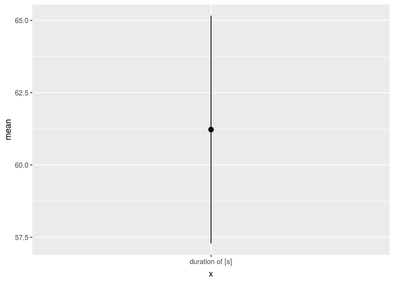
  #geom_errorbar() # For pure line
  #geom_linerange() # For line with borders
2.2 One sample t-test
In some article I found out that mean [s] duration for Chineese is 56 ms. Is the data from [Hau 2007] provides statistically significant difference?
- define H\(_0\): \(\bar{x} = \mu_o\)
- define H\(_1\): \(\bar{x} \ne \mu_o\)
- define p-value

- in most scince fields it is used p-value 0.05
- provide test
\[t = \frac{\bar{x}-\mu_0}{\sigma/\sqrt{n}}\]
\(\sigma\) — standard deviation
homo %>%
  summarise(t_statistics = (mean(s.duration.ms)-56)/(sd(s.duration.ms)/sqrt(n())),
            df = n() - 1,
p_value = 2*pt(-abs(t_statistics),df=df))t.test(homo$s.duration.ms, mu = 56)##
## One Sample t-test
##
## data: homo$s.duration.ms
## t = 2.5997, df = 13, p-value = 0.02202
## alternative hypothesis: true mean is not equal to 56
## 95 percent confidence interval:
## 56.88292 65.56565
## sample estimates:
## mean of x
## 61.224292.3 Normality
one sample t-test assumes:
- normal destribution of data
How to check?
homo %>%
  ggplot(aes(s.duration.ms))+
  geom_density()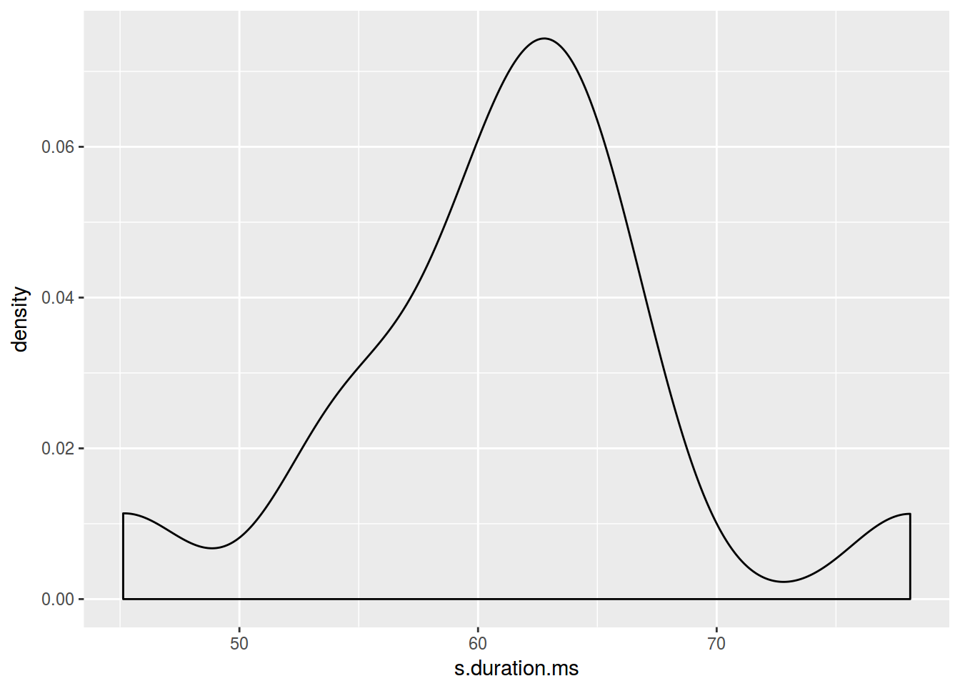
library(sm)
sm.density(homo$s.duration.ms, model = "Normal", col.band="yellowgreen")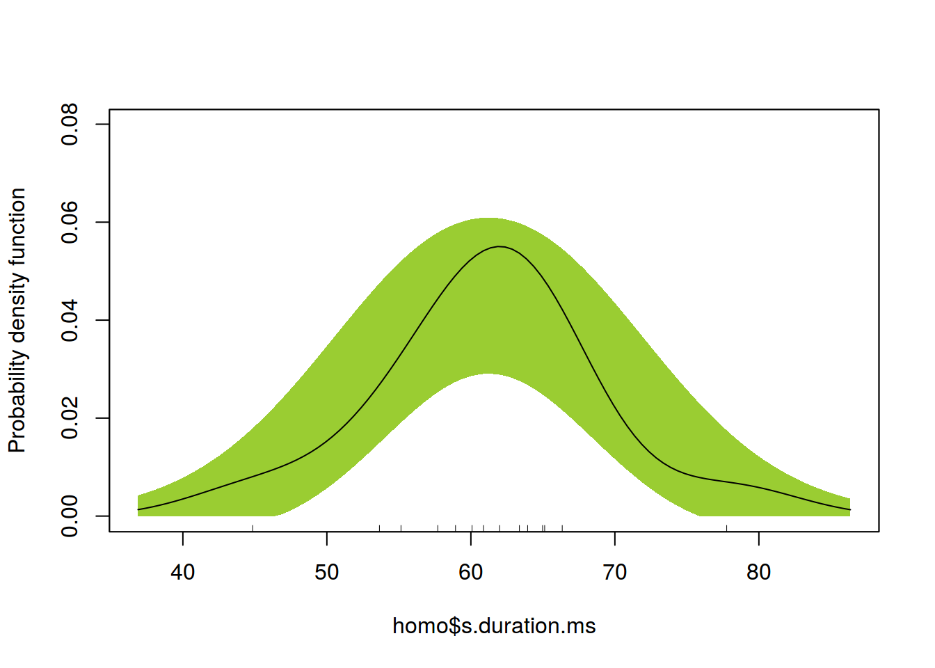
homo %>%
  ggplot(aes(sample = s.duration.ms))+
  geom_qq()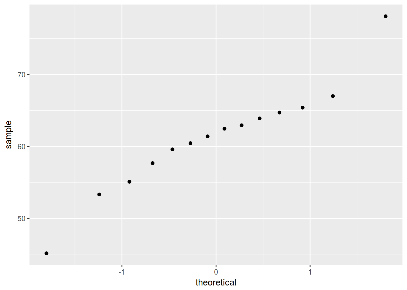
2.5 Wilcoxon test
What if your data is not normally distributed?
wilcox.test(homo$s.duration.ms, mu = 56)##
## Wilcoxon signed rank test
##
## data: homo$s.duration.ms
## V = 89, p-value = 0.02026
## alternative hypothesis: true location is not equal to 563. Two sample test
3.1 Two sample t-test
What if we have two samples?
t.test(s.duration.ms~orientation, data = homo)##
## Welch Two Sample t-test
##
## data: s.duration.ms by orientation
## t = -1.4263, df = 11.994, p-value = 0.1793
## alternative hypothesis: true difference in means is not equal to 0
## 95 percent confidence interval:
## -13.945621 2.911336
## sample estimates:
## mean in group hetero mean in group homo
## 58.46571 63.982863.2 Paired t-test
What if we samples are dependent?
dft.test(df$before, df$after, paired = TRUE)##
## Paired t-test
##
## data: df$before and df$after
## t = 10.919, df = 31, p-value = 3.765e-12
## alternative hypothesis: true difference in means is not equal to 0
## 95 percent confidence interval:
## 2.598141 3.791602
## sample estimates:
## mean of the differences
## 3.1948713.3 Wilcoxon test
wilcox.test(s.duration.ms~orientation, data = homo)##
## Wilcoxon rank sum test
##
## data: s.duration.ms by orientation
## W = 16, p-value = 0.3176
## alternative hypothesis: true location shift is not equal to 0wilcox.test(df$before, df$after, paired = TRUE)##
## Wilcoxon signed rank test
##
## data: df$before and df$after
## V = 526, p-value = 1.397e-09
## alternative hypothesis: true location shift is not equal to 04. Multiple sample tests → next lecture
5. Multiple comparisons problem
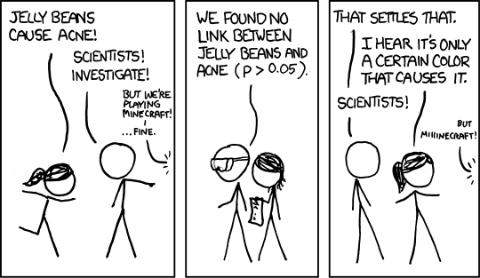
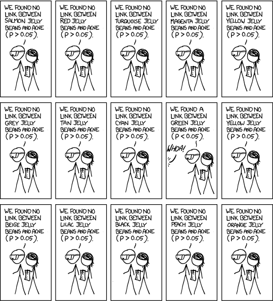

xkcd Significant. Explonation. This colled: data dredging, data fishing, data snooping, equation fitting, p-hacking…
If m independent comparisons are performed, the family-wise error rate (FWER), is given by
\[\alpha = 1 - (1 - \alpha_{for\ each\ pair})^m\] \[\alpha = 1 - (1 - 0.05)^{21} = 1- 0.34 = 0.66\]
5.1 Adjustment for multiple tests
x <- c(0.04, 0.03, 0.01)
p.adjust(x, method = 'bonferroni') # Bonferroni correction
## [1] 0.12 0.09 0.03p.adjust(x, method = 'holm')## [1] 0.06 0.06 0.03p.adjust(x, method = 'BH')## [1] 0.04 0.04 0.03p.adjust(x, method = 'BY')## [1] 0.07333333 0.07333333 0.05500000For conclusion
p-value is not so loved anymore…
- it is misunderstood all the time [Gigerenzer 2004], [Goodman 2008]
p-value < 0.05 is not strong evidence [Sterne, Smith 2001], [Nuzzo et al. 2014], [Wasserstein, Lazar 2016]
- Q: Why do so many colleges and grad schools teach p = 0.05?
- A: Because that’s still what the scientific community and journal editors use.
- Q: Why do so many people still use p = 0.05?
- A: Because that’s what they were taught in college or grad school from (Wasserstein, Lazar 2016)
