5 R packages for phonetics

5.1 `phonfieldwork`

We will work with examples from Abaza and will try to end up with something like this:

5.1.1 Befor we start

I expect you

to install tidyverse and phonfieldwork:

install.packages(c("tidyverse", "rmarkdown", "phonfieldwork"))

load the library:

library(phonfieldwork)

I will use the following version of the package:

packageVersion("phonfieldwork")

[1] '0.0.12'

download files for todays seminar:
- first file
- second file

5.1.2 Philosophy of the `phonfieldwork` package

Most phonetic research consists of the following steps:

Formulate a research question. Think of what kind of data is necessary to answer this question, what is the appropriate amount of data, what kind of annotation you will do, what kind of statistical models and visualizations you will use, etc.
Create a list of stimuli.
Elicite list of stimuli from speakers who signed an Informed Consent statement, agreeing to participate in the experiment to be recorded on audio and/or video. Keep an eye on recording settings: sampling rate, resolution (bit), and number of channels should be the same across all recordings.
Annotate the collected data.
Extract the collected data.
Create visualizations and evaluate your statistical models.
Report your results.
Publish your data.

The phonfieldwork package is created for helping with items 3, partially with 4, and 5 and 8.

To make the automatic annotation of data easier, I usually record each stimulus as a separate file. While recording, I carefully listen to my consultants to make sure that they are producing the kind of speech I want: three isolated pronunciations of the same stimulus, separated by a pause and contained in a carrier phrase. In case a speaker does not produce three clear repetitions, I ask them to repeat the task, so that as a result of my fieldwork session I will have:

a collection of small soundfiles (video) with the same sampling rate, resolution (bit), and number of channels
a list of succesful and unsuccesful attempts to produce a stimulus according to my requirements (usually I keep this list in a regular notebook)

5.1.3 Make a list of your stimuli

First we need to create a list of stimuli. We want to record two Abaza words from speakers (in real life word lists are much longer).

my_stimuli_df <- read.csv("https://raw.githubusercontent.com/agricolamz/2022_HSE_m_Instrumental_phonetics/master/data/my_stimuli_df.csv")
my_stimuli_df

It is also possible to store your list as a column in an .xls or xlsx file and read it into R using the read_xls or read_xlsx functions from the readxl package. If the package readxl is not installed on your computer, you can install it using install.packages("readxl").

5.1.4 Create a presentation based on a list of stimuli

You can show a native speaker your stimuli one by one or not show them the stimuli but ask them to pronounce a certain stimulus or its translation. I use presentations to collect all stimuli in a particular order without the risk of omissions.

When the list of stimuli is loaded into R, you can create a presentation for elicitation. It is important to define an output directory, so in the following example I use the getwd() function, which returns the path to the current working directory. You can set any directory as your current one using the setwd() function. It is also possible to provide a path to your intended output directory with output_dir (e. g. “/home/user_name/…”). This command (unlike setwd()) does not change your working directory.

create_presentation(stimuli = my_stimuli_df$stimuli,
                    output_file = "first_example",
                    output_dir = "sounds/")

As a result, a file “first_example.html” was created in the output folder. You can change the name of this file by changing the output_file argument. The .html file now looks as follows:

https://agricolamz.github.io/2022_HSE_m_Instrumental_phonetics/additional/first_example.html

It is also possible to change the output format, using the output_format argument. By dafault it is “html”, but you can also use “pptx”. There is also an additional argument translations, where you can provide translations for stimuli in order that they appeared near the stimuli on the slide.

create_presentation(stimuli = my_stimuli_df$stimuli, 
                    translations = my_stimuli_df$translation,
                    output_file = "second_example",
                    output_dir = "sounds/")

https://agricolamz.github.io/2022_HSE_m_Instrumental_phonetics/additional/second_example.html

5.1.5 Rename collected data

After collecting data and removing soundfiles with unsuccesful elicitations, one could end up with the following structure:

sounds
├── 01.wav
└── 02.wav

rename_soundfiles(stimuli = my_stimuli_df$stimuli,
                  prefix = "s1_",
                  path = "sounds/examples/")

You can find change correspondences in the following file:
/home/agricolamz/work/materials/2022_HSE_m_instrumental_phonetics/materials/sounds/examples/backup/logging.csv

As a result, you obtain the following structure:

sounds
├── 1_s1_ba.wav
├── 2_s1_bzə.wav
└── backup
    ├── 01.wav
    ├── 02.wav
    └── logging.csv

The rename_soundfiles() function created a backup folder with all of the unrenamed files, and renamed all files using the prefix provided in the prefix argument. There is an additional argument backup that can be set to FALSE (it is TRUE by default), in case you are sure that the renaming function will work properly with your files and stimuli, and you do not need a backup of the unrenamed files. There is also an additional argument logging (TRUE by default) that creates a logging.csv file in the backup folder (or in the original folder if the backup argument has value FALSE) with the correspondences between old and new names of the files. Here is the contence of the logging.csv:

5.1.6 Merge all data together

After all the files are renamed, you can merge them into one. Remmber that sampling rate, resolution (bit), and number of channels should be the same across all recordings. It is possible to resample files with the resample() function from the package biacoustics.

concatenate_soundfiles(path = "sounds/examples/",
                       result_file_name = "s1_all")

This comand creates a new soundfile s1_all.wav and an asociated Praat TextGrid s1_all.TextGrid:

├── 1_s1_ba.wav
├── 2_s1_bzə.wav
├── s1_all.TextGrid
├── s1_all.wav
└── backup
    ├── 01.wav
    ├── 02.wav
    └── logging.csv

The resulting file can be parsed with Praat:

Sometimes recorded sounds do not have any silence at the beginning or the end, so after the merging the result utterances will too close to each other. It is possible to fix using the argument separate_duration of the concatenate_soundfiles() function: just put the desired duration of the separator in seconds.

It is not kind of task that could occur within phonfieldwork philosophy, but it also possible to merge multiple .TextGrids with the same tier structure using concatente_textgrids() function.

5.1.7 Annotate your data

It is possible to annotate words using an existing annotation:

my_stimuli_df$stimuli

[1] "ba"  "bzə"

annotate_textgrid(annotation = my_stimuli_df$stimuli,
                  textgrid = "sounds/examples/s1_all.TextGrid")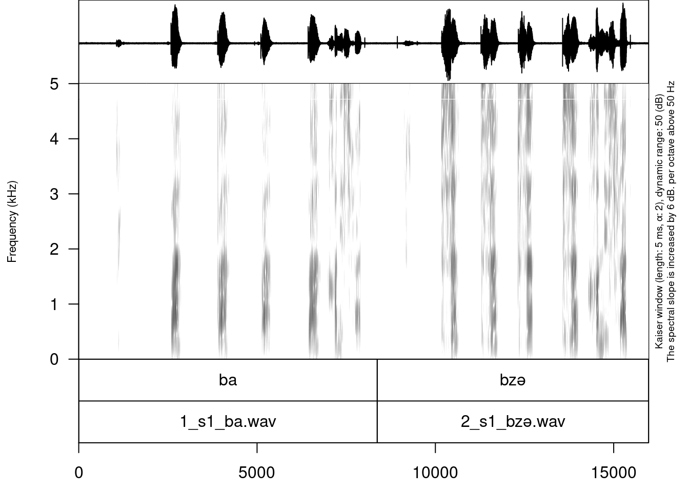

As you can see in the example, the annotate_textgrid() function creates a backup of the tier and adds a new tier on top of the previous one. It is possible to prevent the function from doing so by setting the backup argument to FALSE.

annotate_textgrid(annotation = my_stimuli_df$translation,
                  textgrid = "sounds/examples/s1_all.TextGrid",
                  tier = 2, 
                  backup = FALSE)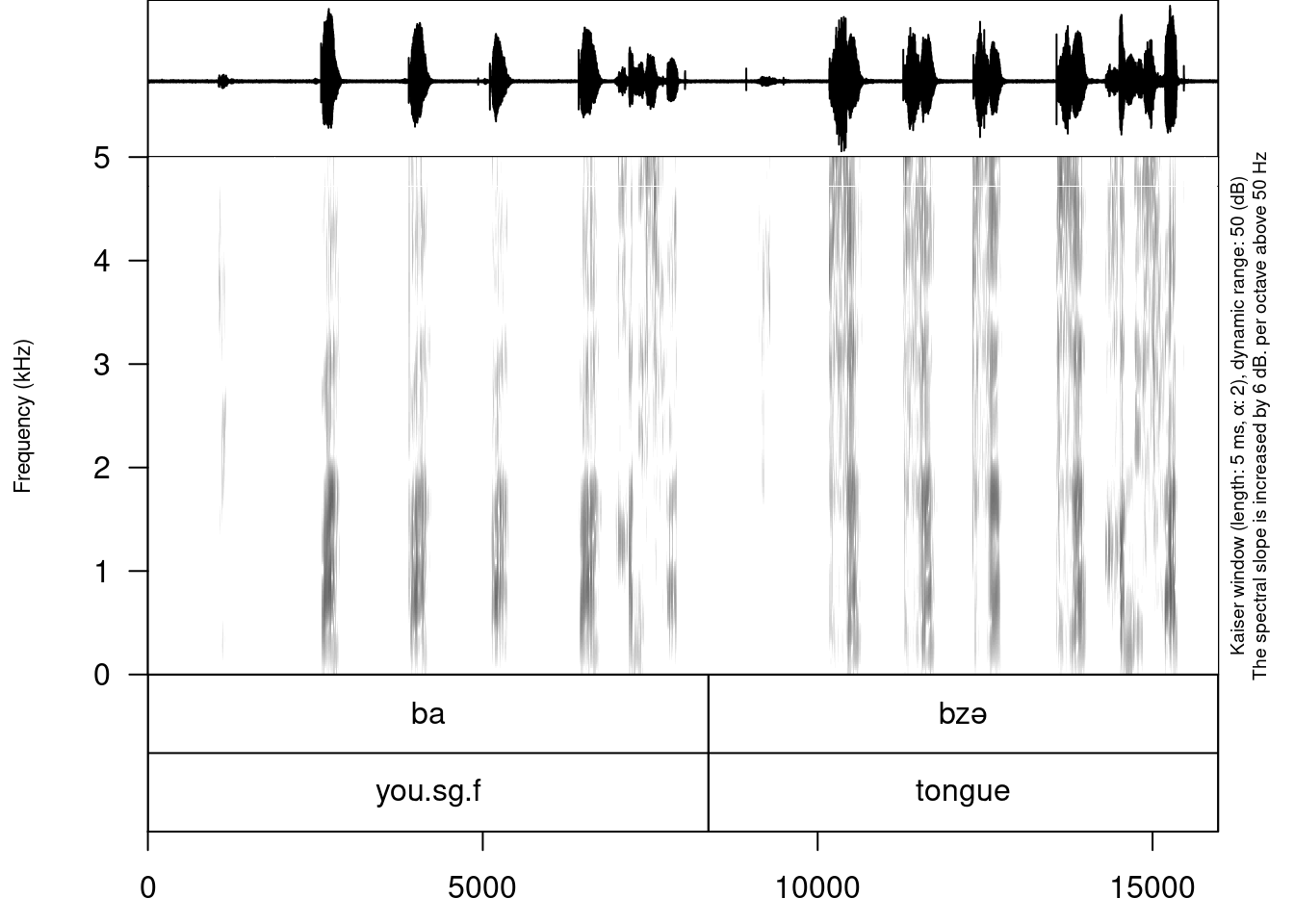

Imagine that we are interested in annotation of vowels. The most common solution will be open Praat and create new annotations. But it is also possible to create them in advance using subannotations. The idea that you choose some baseline tier that later will be automatically cutted into smaller pieces on the other tier.

create_subannotation(textgrid = "sounds/examples/s1_all.TextGrid",
                     tier = 1, # this is a baseline tier
                     n_of_annotations = 9) # how many empty annotations per unit?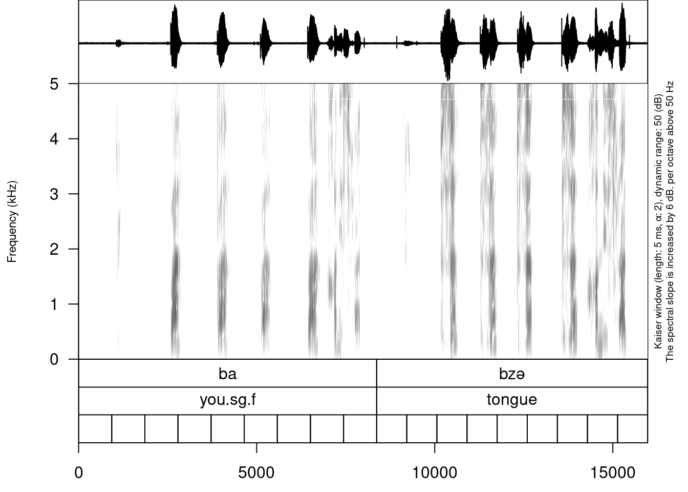

It is worth mentioning that if you want to have different number of subannotation per unit, you can pass a vector of required numbers to n_of_annotations argument.

After the creation of subannotations, we can annotate created tier:

annotate_textgrid(annotation = c("", "a", "", "a", "", "a", "", "a", "",
                                 "", "ə", "", "ə", "", "ə", "", "ə", ""),
                  textgrid = "sounds/examples/s1_all.TextGrid",
                  tier = 3,
                  backup = FALSE)

We can also add some tier for uterance annotation:

create_subannotation(textgrid = "sounds/examples/s1_all.TextGrid",
                     tier = 1,
                     n_of_annotations = 9)
annotate_textgrid(annotation = c("", "u_1", "", "u_2", "", "u_3", "", "cf", "",
                                 "", "u_1", "", "u_2", "", "u_3", "", "cf", ""),
                  textgrid = "sounds/examples/s1_all.TextGrid",
                  tier = 4,
                  backup = FALSE)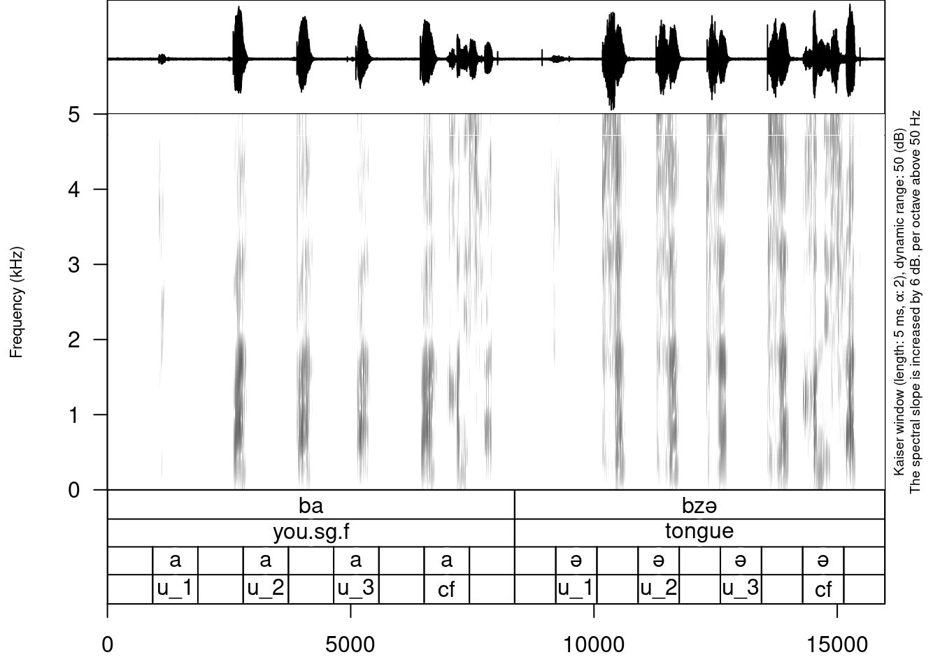

You can see that we created a third tier with annotation. The only thing left is to move annotation boundaries in Praat (this can not be automated):

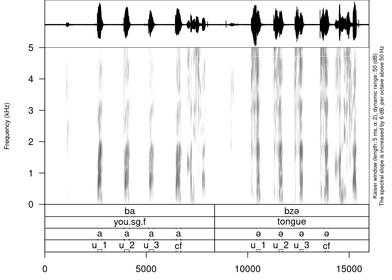
Here you can download the result .TextGrid (you can press Ctrl+S, when you open it).

5.1.8 Extracting your data

First, it is important to create a folder where all of the extracted files will be stored:

dir.create("sounds/examples/s1_sounds")

It is possible to extract all annotated files based on an annotation tier:

extract_intervals(file_name = "sounds/examples/s1_all.wav",
                  textgrid = "sounds/examples/s1_all.TextGrid",
                  tier = 3,
                  path = "sounds/examples/s1_sounds/",
                  prefix = "s1_")

sounds/examples
├── 1_s1_ba.wav
├── 2_s1_bzə.wav
├── s1_all.TextGrid
├── s1_all.wav
├── backup
│   ├── 01.wav
│   ├── 02.wav
│   └── logging.csv
└── s1_sounds
    ├── 01_s1_a.wav
    ├── 02_s1_a.wav
    ├── 03_s1_a.wav
    ├── 04_s1_a.wav
    ├── 05_s1_ə.wav
    ├── 06_s1_ə.wav
    ├── 07_s1_ə.wav
    └── 08_s1_ə.wav

5.1.9 Visualizing your data

It is possible to view an oscilogram and spetrogram of any soundfile:

draw_sound(file_name = "sounds/examples/s1_sounds/01_s1_a.wav")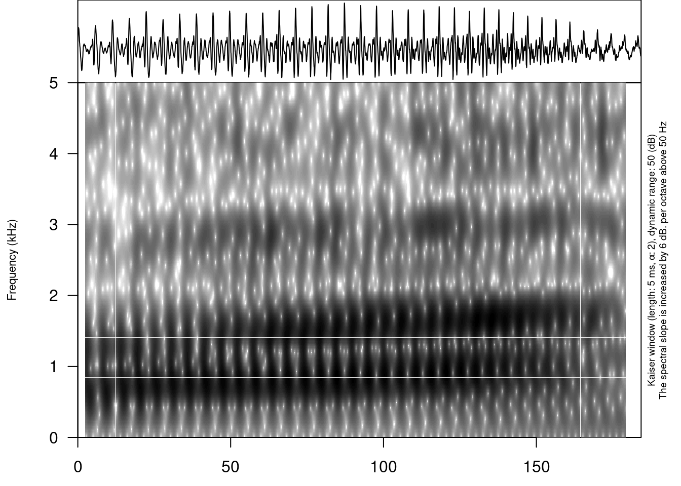

There are additional parameters:

title – the title for the plot
from – time in seconds at which to start extraction
to – time in seconds at which to stop extraction
zoom – time in seconds for zooming spectrogram
text_size – size of the text on the plot
annotation – the optional file with the TextGrid’s file path or dataframe with annotations (see the section 5.)
freq_scale – the measure of the frequency: can be “Hz” or “kHz”.
frequency_range – the frequency range to be displayed for the spectrogram
dynamic_range – values greater than this many dB below the maximum will be displayed in the same color
window_length – the desired length in milliseconds for the analysis window
window – window type (can be “rectangular”, “hann”, “hamming”, “cosine”, “bartlett”, “gaussian”, and “kaiser”)
preemphasisf – Preemphasis of 6 dB per octave is added to frequencies above the specified frequency. For no preemphasis (important for bioacoustics), set to a 0.
spectrum_info – logical value, if FALSE won’t print information about spectorgram on the right side of the plot.
output_file – the name of the output file
output_width – the width of the device
output_height – the height of the device
output_units – the units in which height and width are given. This can be “px” (pixels, which is the default value), “in” (inches), “cm” or “mm”.

It is really important in case you have a long file not to draw the whole file, since it won’t fit into the RAM of your computer. So you can use from and to arguments in order to plot the fragment of the sound and annotation:

draw_sound("sounds/examples/s1_all.wav",
           "sounds/examples/s1_all.TextGrid")

5.1.10 Read linguistic files into R

The phonfieldwork package provides also several methods for reading different file types into R. This makes it possible to analyze them and convert into .csv files (e. g. using the write.csv() function). The main advantage of using those functions is that all of them return data.frames with columns (time_start, time_end, content and source). This make it easer to use the result in the draw_sound() function that make it possible to visualise all kind of sound annotation systems.

file .TextGrid from Praat; see also rPraat and textgRid packages

df <- textgrid_to_df("sounds/examples/s1_all.TextGrid")
df

library(tidyverse)
df %>% 
  filter(tier_name == "vowels" | 
           tier_name == "uterances", 
         content != "") %>% 
  mutate(duration =  time_end - time_start) %>% 
  select(content, tier_name, duration) %>% 
  pivot_wider(names_from = tier_name,
              values_from = content) ->
  results

results %>% 
  ggplot(aes(vowels, duration))+
  geom_point()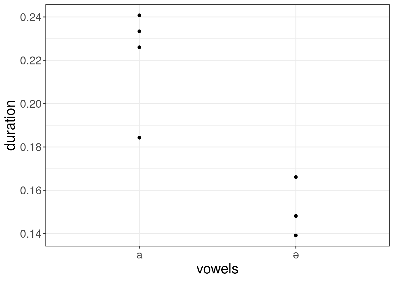

5.1.11 Documentation

You can find the whole documentation for phonfieldwork here.

If you will use the package it make sense to cite it:

citation("phonfieldwork")


Moroz G (2020). _Phonetic fieldwork and experiments with phonfieldwork
package_. <URL: https://CRAN.R-project.org/package=phonfieldwork>.

A BibTeX entry for LaTeX users is

  @Manual{,
    title = {Phonetic fieldwork and experiments with phonfieldwork package},
    author = {George Moroz},
    year = {2020},
    url = {https://CRAN.R-project.org/package=phonfieldwork},
  }

5.2 `ipa`

Converts character vectors between phonetic representations. Supports IPA (International Phonetic Alphabet), X-SAMPA (Extended Speech Assessment Methods Phonetic Alphabet), and ARPABET (used by the CMU Pronouncing Dictionary).

library(ipa)
convert_phonetics('%hE"loU', from = "xsampa", to = "ipa")

[1] "ˌhɛˈloʊ"

If you will use the package it make sense to cite it:

citation("ipa")


To cite ipa in publications use:

  Alexander Rossell Hayes (2020). ipa: convert between phonetic
  alphabets. R package version 0.1.0.
  https://github.com/rossellhayes/ipa

A BibTeX entry for LaTeX users is

  @Manual{,
    title = {ipa: convert between phonetic alphabets},
    author = {Rossell Hayes and {Alexander}},
    year = {2020},
    note = {R package version 0.1.0},
    url = {https://github.com/rossellhayes/ipa},
  }

5.3 `phonTools`

This package contains tools for the organization, display, and analysis of the sorts of data frequently encountered in phonetics research and experimentation, including the easy creation of IPA vowel plots, and the creation and manipulation of WAVE audio files.

This package is usefull, since it provides some datasets:

pb52 — Peterson & Barney (1952) Vowel Data (1520 rows)
f73 — Fant (1973) Swedish Vowel Data (10 rows)
p73 — Pols et al. (1973) Dutch Vowel Data (12 rows)
b95 — Bradlow (1995) Spanish Vowel Data (5 rows)
h95 — Hillenbrand et al. (1995) Vowel Data (1668 rows)
a96 — Aronson et al. (1996) Hebrew Vowel Data (10 rows)
y96 — Yang (1996) Korean Vowel Data (20 rows)
f99 — Fourakis et al. (1999) Greek Vowel Data (5 rows)
t07 — Thomson (2007) Vowel Data (20 rows)

In order to load them you need to follow these steps:

library(phonTools)
data(h95)
h95

As you see vowel column is in X-SAMPA. In order to use it we need to recode it:

library(tidyverse)
h95 %>% 
  mutate(vowel = convert_phonetics(vowel, from = "xsampa", to = "ipa")) %>%
  ggplot(aes(f2, f1, label = vowel, color = vowel))+
  stat_ellipse()+
  geom_text()+
  scale_x_reverse()+
  scale_y_reverse()+
  coord_fixed()+
  facet_wrap(~type)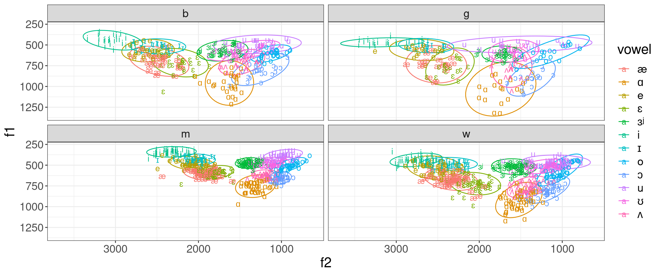

It also make sense to use normalization for vowels:

h95 %>% 
  mutate(vowel = convert_phonetics(vowel, from = "xsampa", to = "ipa")) %>%
  group_by(speaker) %>% 
  mutate(f1 = scale(f1),
         f2 = scale(f2)) %>% 
  ggplot(aes(f2, f1, label = vowel, color = vowel))+
  stat_ellipse()+
  geom_text()+
  scale_x_reverse()+
  scale_y_reverse()+
  facet_wrap(~type)+
  labs(title = "Normalized vowels")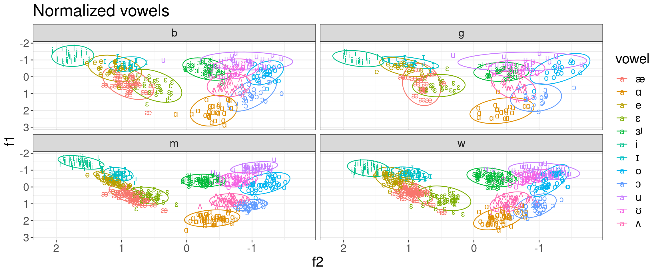

If you will use the package it make sense to cite it:

citation("phonTools")


To cite package 'phonTools' in publications use:

  Santiago Barreda (2015). phonTools: Functions for phonetics in R. R
  package version 0.2-2.1.

A BibTeX entry for LaTeX users is

  @Manual{,
    title = {phonTools: Functions for phonetics in R.},
    author = {Santiago Barreda},
    year = {2015},
    note = {R package version 0.2-2.1},
  }

5.4 `vowels`

Procedures for the manipulation, normalization, and plotting of phonetic and sociophonetic vowel formant data. vowels is the backend for the NORM website.

If you will use the package it make sense to cite it:

citation("vowels")


To cite package 'vowels' in publications use:

  Tyler Kendall and Erik R. Thomas (2018). vowels: Vowel Manipulation,
  Normalization, and Plotting. R package version 1.2-2.
  https://CRAN.R-project.org/package=vowels

A BibTeX entry for LaTeX users is

  @Manual{,
    title = {vowels: Vowel Manipulation, Normalization, and Plotting},
    author = {Tyler Kendall and Erik R. Thomas},
    year = {2018},
    note = {R package version 1.2-2},
    url = {https://CRAN.R-project.org/package=vowels},
  }

ATTENTION: This citation information has been auto-generated from the
package DESCRIPTION file and may need manual editing, see
'help("citation")'.

5.5 `rPraat`

This is a package for reading, writing and manipulating Praat objects like TextGrid, PitchTier, Pitch, IntensityTier, Formant, Sound, and Collection files. You can find the demo for rPraat here.

If you will use the package it make sense to cite it:

citation("rPraat")


To cite rPraat in publications use:

  Bořil, T., & Skarnitzl, R. (2016). Tools rPraat and mPraat. In P.
  Sojka, A. Horák, I. Kopeček, & K. Pala (Eds.), Text, Speech, and
  Dialogue (pp. 367-374). Springer International Publishing.

A BibTeX entry for LaTeX users is

  @InProceedings{,
    author = {Tomáš Bořil and Radek Skarnitzl},
    editor = {Petr Sojka and Aleš Horák and Ivan Kopeček and Karel Pala},
    booktitle = {Text, Speech, and Dialogue: 19th International Conference, TSD 2016, Brno, Czech Republic, September 12-16, 2016, Proceedings},
    publisher = {Springer International Publishing},
    address = {Cham},
    year = {2016},
    title = {Tools rPraat and mPraat},
    pages = {367--374},
    isbn = {978-3-319-45510-5},
    doi = {10.1007/978-3-319-45510-5_42},
    url = {http://dx.doi.org/10.1007/978-3-319-45510-5_42},
  }

5.6 `speakr`

This package allows running Praat scripts from R and it provides some wrappers for basic plotting.

On macOS, Linux and Windows, the path to Praat is set automatically to the default installation path. If you have installed Praat in a different location, or if your operating system is not supported, you can set the path to Praat with options(speakr.praat.path).

For example:

options(speakr.praat.path = "./custom/praat.exe")

If you use rstudio.cloud you need to upload the unziped file of Linux version of Praat and provide path to it within the options():

options(speakr.praat.path = "/cloud/projects/praat")

You can either run this command every time you start a new R session, or you can add the command to your .Rprofile.

If you run into the problem with permisions run the following command:

system("chmod 700 /cloud/projects/praat")

As an example I will use the following data:

├── get-formants-args.praat
├── s1_all.TextGrid
└── s1_all.wav

Here are the s1_all.TextGrid, s1_all.wav and the get-formants-args.praat:

sound = Read from file: "s1_all.wav"
formant = To Formant (burg): 0, 5, 5000, 0.05, 50
textgrid = Read from file: "s1_all.TextGrid"
header$ = "vowel,F1,F2,F3"
writeInfoLine: header$

form Get formants
    choice Measure 1
        button Hertz
        button Bark
    real Window_(sec) 0.03
endform

if measure == 1
    measure$ = "Hertz"
else
    measure$ = "Bark"
endif

selectObject: textgrid
intervals = Get number of intervals: 3

for interval to intervals - 1
    label$ = Get label of interval: 3, interval
    if label$ != ""
        start = Get start time of interval: 3, interval
        start = start + window
        end = Get end time of interval: 3, interval
        end = end - window
        vowel$ = Get label of interval: 3, interval

        selectObject: formant
        f1 = Get mean: 1, start, end, measure$
        f2 = Get mean: 2, start, end, measure$
        f3 = Get mean: 3, start, end, measure$

        resultLine$ = "'vowel$','f1','f2','f3'"
        appendInfoLine: resultLine$
        selectObject: textgrid
    endif
endfor

In order to use it you need to provide path to the script:

library(speakr)

Praat found at /usr/bin/praat

praat_run("sounds/speakr/get-formants-args.praat", 
          "Hertz", 0.03, capture = TRUE)

[1] "vowel,F1,F2,F3\na,832.4811857289797,1530.407389678815,2174.814335788099\na,775.505720968018,1368.2558211702246,2509.084391503502\na,833.9754988486553,1430.9906341641104,2375.2400400500196\na,863.5056920837876,1546.8857016095715,2890.4894773135247\nə,723.6246579247697,1689.4016617222446,2873.1991954244213\nə,717.2753390554032,1675.2062036645505,2745.5586414564323\nə,758.8975215666187,1679.0831544665587,2698.956344303706\nə,711.4372573263009,1685.1137747815465,3031.5963943557826"

As you see the result is file in a .csv format. We can use the following code in order to visualise it:

library(tidyverse)
praat_run("sounds/speakr/get-formants-args.praat", 
          "Hertz", 0.03, capture = TRUE) %>% 
  read_csv() ->
  abaza_formants

Rows: 8 Columns: 4
── Column specification ────────────────────────────────────────────────────────
Delimiter: ","
chr (1): vowel
dbl (3): F1, F2, F3

ℹ Use `spec()` to retrieve the full column specification for this data.
ℹ Specify the column types or set `show_col_types = FALSE` to quiet this message.

abaza_formants %>% 
  ggplot(aes(F2, F1, label = vowel, color = vowel))+
  geom_text()+
  scale_x_reverse()+
  scale_y_reverse()+
  coord_fixed()+
  labs(title = "Example of Abaza vowels")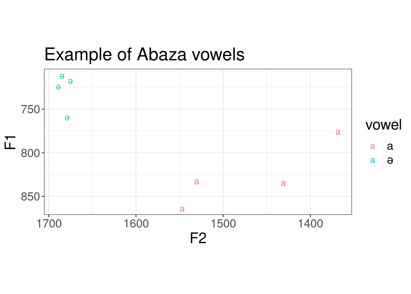

Actually we can merge data on formants and data on duration together:

library(phonfieldwork)

abaza_duration <- textgrid_to_df("sounds/speakr/s1_all.TextGrid")
abaza_duration %>% 
  filter(tier == 3,
         content != "") %>% 
  mutate(duration = time_end - time_start) %>% 
  select(content, duration) ->
  abaza_duration

abaza_duration

abaza_formants %>% 
  bind_cols(abaza_duration) %>% 
  ggplot(aes(F2, F1, label = vowel, color = vowel, size = duration))+
  geom_text()+
  scale_x_reverse()+
  scale_y_reverse()+
  coord_fixed()+
  labs(title = "Example of Abaza vowels")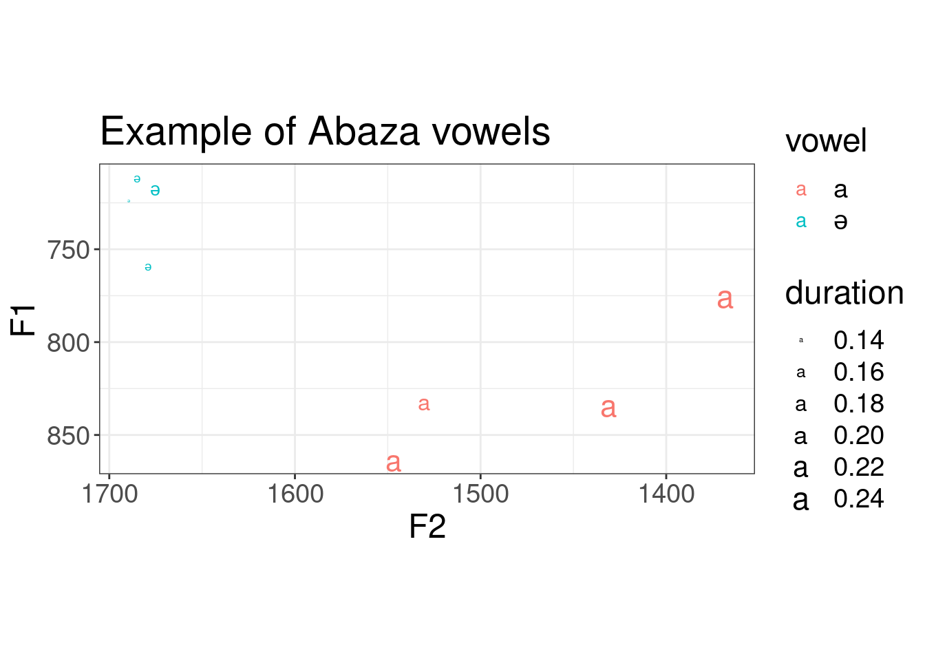

If you will use the package it make sense to cite it:

citation("speakr")


To cite package 'speakr' in publications use:

  Stefano Coretta (2021). speakr: A Wrapper for the Phonetic Software
  'Praat'. R package version 3.2.0.
  https://CRAN.R-project.org/package=speakr

A BibTeX entry for LaTeX users is

  @Manual{,
    title = {speakr: A Wrapper for the Phonetic Software 'Praat'},
    author = {Stefano Coretta},
    year = {2021},
    note = {R package version 3.2.0},
    url = {https://CRAN.R-project.org/package=speakr},
  }

5 R packages for phonetics

5.1 phonfieldwork

5.1.1 Befor we start

5.1.2 Philosophy of the phonfieldwork package

5.1.3 Make a list of your stimuli

5.1.4 Create a presentation based on a list of stimuli

5.1.5 Rename collected data

5.1.6 Merge all data together

5.1.7 Annotate your data

5.1.8 Extracting your data

5.1.9 Visualizing your data

5.1.10 Read linguistic files into R

5.1.11 Documentation

5.2 ipa

5.3 phonTools

5.4 vowels

5.5 rPraat

5.6 speakr

5.1 `phonfieldwork`

5.1.2 Philosophy of the `phonfieldwork` package

5.2 `ipa`

5.3 `phonTools`

5.4 `vowels`

5.5 `rPraat`

5.6 `speakr`