Chapter 2 Introduction to R language

Since this book includes a lot of R code examples, this chapter will describe some basics for those, who is not familiar with R. For purposes of understanding R code in this book you don’t need any deep knowledge of R. In case you want to learn more, there are a lot of good books on it. I will list only few of them:

2.1 Instalation

2.1.1 R instalation

To download R, go to CRAN. Don’t try to pick a mirror that’s close to you, instead it is better to use the cloud mirror, https://cloud.r-project.org.

2.1.2 RStudio

RStudio is an integrated development environment, or IDE, for R programming. There are two possibilities for using it:

type R code in the R console pane, and press enter to run it;
type R code in the Code editor pane, and press Control/Command + Enter to run selected part. It is easier to correct and it is possible to save the result as a script.

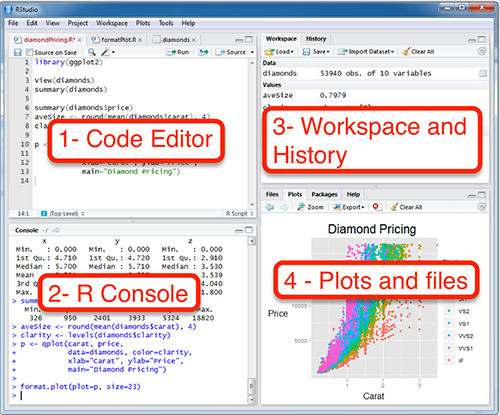
Figure 2.1: RStudio layout

When you first launch RStudio it is more likely, that you won’t see the Code Editor pane. It is possible to decrease R Console pane on icons in the pane’s right upper corner.

Everything from this book will be availible without RStudio instalation. There are a lot of possibilities to work with R not using RStudio such as R console, command line, Jupyter Notebook, some plugins for working in Sublime, Vim, Emacs, Atom, Notepad++ and other programming text editors.

2.1.3 RStuio cloud

It is also possible not to install anything on your own PC, using RStudio Cloud, a web-based interface for Rstudio and R. In RStudio Cloud it is also possible to share your R projects and collaborate with a select group in a private space. RStudio Cloud is currently free to use, but soon there will be free and paid options.

2.2 Basic elements, variables, vectors, dataframe

2.2.1 Basic elements

[1] 7

-5.7

[1] -5.7

"bonjour"

[1] "bonjour"

"bon mot"

[1] "bon mot"

TRUE

[1] TRUE

FALSE

[1] FALSE

2.2.2 Arithmetic operations

7+7

[1] 14

21-8

[1] 13

4*3

[1] 12

12/4

[1] 3

4^3

[1] 64

4**3

[1] 64

sum(1, 2,3, 4)

[1] 10

prod(1, 2,3, 4)

[1] 24

log(1)

[1] 0

log(100, base = 10)

[1] 2

pi

[1] 3.141593

exp(5)

[1] 148.4132

sin(13)

[1] 0.420167

cos(13)

[1] 0.9074468

2.2.3 Variables

my_var <- 7
my_var

[1] 7

my_var+7

[1] 14

my_var

[1] 7

my_var <- my_var + 7

2.2.4 Vectors

5:9

[1] 5 6 7 8 9

11:4

[1] 11 10  9  8  7  6  5  4

numbers <- c(7, 9.9, 24)
multiple_strings <- c("the", "quick", "brown", "fox", "jumps", "over", "the", "lazy", "dog")
one_string <- c("the quick brown fox jumps over the lazy dog")
true_false <- c(TRUE, FALSE, FALSE, TRUE)
length(numbers)

[1] 3

length(multiple_strings)

[1] 9

length(one_string)

[1] 1

2.2.5 Dataframes

my_df <- data.frame(latin = c("a", "b", "c"),
                    cyrillic = c("а", "б", "в"),
                    greek = c("α", "β", "γ"),
                    numbers = c(1:3),
                    is.vowel = c(TRUE, FALSE, FALSE),
                    stringsAsFactors = FALSE)
my_df

  latin cyrillic greek numbers is.vowel
1     a        а     α       1     TRUE
2     b        б     β       2    FALSE
3     c        в     γ       3    FALSE

nrow(my_df)

[1] 3

ncol(my_df)

[1] 5

2.2.6 Indexing

numbers[3]

[1] 24

multiple_strings[9]

[1] "dog"

my_df[2, 3]

[1] "β"

my_df[2,]

  latin cyrillic greek numbers is.vowel
2     b        б     β       2    FALSE

my_df[,3]

[1] "α" "β" "γ"

my_df$is.vowel

[1]  TRUE FALSE FALSE

my_df$is.vowel[2]

[1] FALSE

2.3 Reading files

We can read to R a dataset about Numeral Classifiers from AUTOTYP database.

new_df <- read.csv("https://raw.githubusercontent.com/autotyp/autotyp-data/master/data/Numeral_classifiers.csv")
head(new_df)

  LID NumClass.n NumClass.Presence
1 148          0             FALSE
2  65          0             FALSE
3  75          0             FALSE
4  85          0             FALSE
5 111         NA                NA
6 163          0             FALSE

tail(new_df)

     LID NumClass.n NumClass.Presence
250 1397          0             FALSE
251 2994          5              TRUE
252 2779          0             FALSE
253  192          0             FALSE
254  551          0             FALSE
255 2564          2              TRUE

It could be also a file on your computer, just provide a whole path to the file. Windows users need to change backslashes \ to slashes /.

new_df_2 <- read.csv("/home/agricolamz/my_file.csv")

2.4 Writing files from R

write.csv(new_df_2, "/home/agricolamz/my_new_file.csv",
          row.names = FALSE)

2.5 Missing data

In R, missing values are represented by the symbol NA (not available).

is.na(new_df$NumClass.Presence)

  [1] FALSE FALSE FALSE FALSE  TRUE FALSE FALSE FALSE FALSE FALSE FALSE
 [12] FALSE FALSE FALSE FALSE FALSE FALSE FALSE FALSE FALSE FALSE FALSE
 [23] FALSE FALSE FALSE FALSE FALSE FALSE FALSE FALSE FALSE FALSE FALSE
 [34] FALSE FALSE FALSE FALSE FALSE FALSE FALSE FALSE FALSE FALSE FALSE
 [45] FALSE FALSE FALSE FALSE FALSE FALSE FALSE FALSE FALSE FALSE FALSE
 [56] FALSE FALSE FALSE FALSE FALSE FALSE FALSE FALSE FALSE FALSE FALSE
 [67] FALSE FALSE FALSE FALSE FALSE FALSE FALSE FALSE FALSE FALSE FALSE
 [78] FALSE FALSE FALSE FALSE FALSE FALSE FALSE FALSE FALSE FALSE FALSE
 [89] FALSE FALSE FALSE FALSE FALSE FALSE FALSE FALSE FALSE FALSE FALSE
[100] FALSE FALSE FALSE FALSE FALSE FALSE  TRUE FALSE FALSE FALSE FALSE
[111] FALSE FALSE FALSE FALSE FALSE FALSE FALSE FALSE FALSE FALSE FALSE
[122] FALSE FALSE FALSE FALSE FALSE FALSE FALSE FALSE FALSE FALSE FALSE
[133] FALSE FALSE FALSE FALSE FALSE FALSE FALSE FALSE FALSE FALSE FALSE
[144] FALSE FALSE FALSE FALSE FALSE FALSE FALSE FALSE FALSE FALSE FALSE
[155] FALSE FALSE FALSE FALSE FALSE FALSE FALSE FALSE FALSE FALSE  TRUE
[166] FALSE FALSE FALSE FALSE FALSE FALSE FALSE FALSE FALSE FALSE FALSE
[177]  TRUE FALSE FALSE FALSE FALSE FALSE FALSE FALSE  TRUE FALSE FALSE
[188] FALSE FALSE FALSE FALSE FALSE FALSE FALSE FALSE FALSE FALSE FALSE
[199] FALSE FALSE FALSE FALSE FALSE FALSE FALSE FALSE FALSE FALSE FALSE
[210] FALSE FALSE FALSE FALSE FALSE FALSE FALSE FALSE FALSE FALSE FALSE
[221] FALSE FALSE FALSE FALSE FALSE FALSE FALSE FALSE FALSE FALSE FALSE
[232] FALSE FALSE FALSE FALSE FALSE FALSE FALSE FALSE FALSE FALSE FALSE
[243] FALSE FALSE FALSE FALSE FALSE FALSE FALSE FALSE FALSE FALSE FALSE
[254] FALSE FALSE

sum(is.na(new_df$NumClass.Presence))

[1] 5

sum(is.na(new_df))

[1] 22

2.6 How to get help in R

?nchar

2.7 Packages

There are a lot of R packages for solving a lot of different problems. There are two way for install them (you need an internet connection):

packages on CRAN are checked in multiple ways and should be stable

install.packages("lingtypology")

packages on GitHub are NOT checked and could contain anything, but it is the place where all package developers keep the last vertion of they work.

install.packages("devtools")
devtools::install_github("ropensci/lingtypology")

or package file

install.packages("lingtypology",
                 destdir = "/path/to/your/package")

After the package is installed you need to load the package using the following command:

library("lingtypology")

There is a nice picture from Phillips N. D. (2017) YaRrr! The Pirate’s Guide to R:

Figure 2.2: Lamp metaphore