10 Логистическая, порядковая и мультиномиальная регрессия
library(tidyverse)Логистическая (logit, logistic) и мультиномиальная (multinomial) регрессия применяются в случаях, когда зависимая переменная является категориальной:
- с двумя значениями (логистическая регрессия)
- с более чем двумя значениями, упорядоченными в иерархию (порядковая регрессия)
- с более чем двумя значениями (мультиномиальная регрессия)
10.1 Логистическая регрессия
10.1.1 Теория
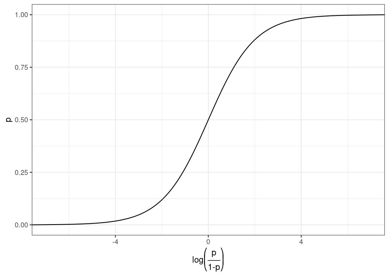
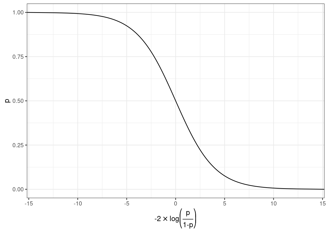
Мы хотим чего-то такого: \[\underbrace{y}_{[-\infty, +\infty]}=\underbrace{\mbox{β}_0+\mbox{β}_1\cdot x_1+\mbox{β}_2\cdot x_2 + \dots +\mbox{β}_k\cdot x_k +\mbox{ε}_i}_{[-\infty, +\infty]}\] Вероятность — отношение количества успехов к общему числу событий: \[p = \frac{\mbox{# успехов}}{\mbox{# неудач} + \mbox{# успехов}}, p \in [0, 1]\] Шансы — отношение количества успехов к количеству неудач: \[odds = \frac{p}{1-p} = \frac{p\mbox{(успеха)}}{p\mbox{(неудачи)}}, odds \in [0, +\infty]\] Натуральный логарифм шансов: \[\log(odds) \in [-\infty, +\infty]\]
Но, что нам говорит логарифм шансов? Как нам его интерпретировать?
tibble(n = 10,
           success = 1:9,
           failure = n - success,
           prob.1 = success/(success+failure),
           odds = success/failure,
           log_odds = log(odds),
           prob.2 = exp(log_odds)/(1+exp(log_odds)))
Как связаны вероятность и логарифм шансов: \[\log(odds) = \log\left(\frac{p}{1-p}\right)\] \[p = \frac{\exp(\log(odds))}{1+\exp(\log(odds))}\]
Логарифм шансов равен 0.25. Посчитайте вероятность успеха:
Как связаны вероятность и логарифм шансов:
10.1.2 Практика
В датасет собрано 19 языков, со следующими переменными:
language— переменная, содержащая языкtone— бинарная переменная, обозначающая наличие тоновlong_vowels— бинарная переменная, обозначающая наличие долгих гласныхstress— бинарная переменная, обозначающая наличие ударенияejectives— бинарная переменная, обозначающая наличие абруптивныхconsonants— переменная, содержащая информацию о количестве согласныхvowels— переменная, содержащая информацию о количестве гласных
phonological_profiles <- read_csv("https://raw.githubusercontent.com/agricolamz/2021_da4l/master/data/phonological_profiles.csv")
glimpse(phonological_profiles)
Rows: 19
Columns: 8
$ language <chr> "Turkish", "Korean", "Tiwi", "Liberia Kpelle", "Tulu", "Ma…
$ tone <lgl> FALSE, FALSE, FALSE, TRUE, FALSE, FALSE, TRUE, FALSE, TRUE…
$ long_vowels <lgl> TRUE, FALSE, FALSE, FALSE, TRUE, FALSE, TRUE, FALSE, TRUE,…
$ stress <lgl> TRUE, TRUE, TRUE, FALSE, FALSE, TRUE, FALSE, TRUE, TRUE, F…
$ ejectives <lgl> FALSE, FALSE, FALSE, FALSE, FALSE, FALSE, FALSE, FALSE, FA…
$ consonants <dbl> 25, 21, 22, 22, 24, 20, 22, 24, 15, 18, 17, 8, 26, 28, 30,…
$ vowels <dbl> 8, 11, 4, 12, 13, 6, 20, 12, 5, 11, 8, 5, 14, 6, 7, 7, 5, …
$ area <chr> "Eurasia", "Eurasia", "Australia", "Africa", "Eurasia", "S…set.seed(42)
phonological_profiles %>%
ggplot(aes(ejectives, consonants))+
geom_boxplot(aes(fill = ejectives), show.legend = FALSE, outlier.alpha = 0)+
# по умолчанию боксплот рисует выбросы, outlier.alpha = 0 -- это отключает
geom_jitter(size = 3)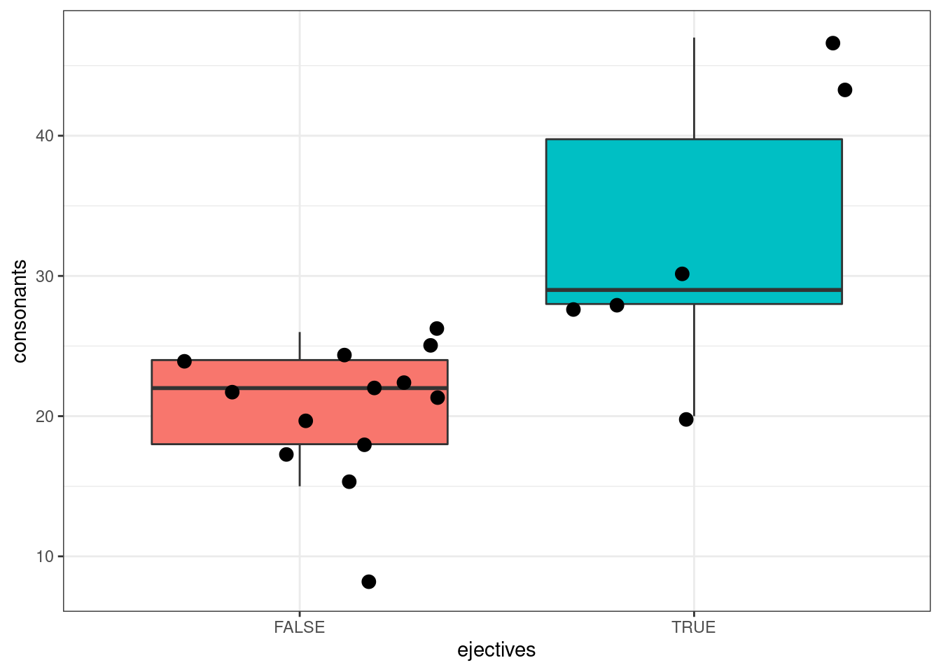
10.1.2.1 Почему не линейную регрессию?
lm_0 <- lm(as.double(ejectives)~1, data = phonological_profiles)
lm_1 <- lm(as.double(ejectives)~consonants, data = phonological_profiles)
lm_0
Call:
lm(formula = as.double(ejectives) ~ 1, data = phonological_profiles)

Coefficients:
(Intercept)
     0.3158
lm_1
Call:
lm(formula = as.double(ejectives) ~ consonants, data = phonological_profiles)

Coefficients:
(Intercept)   consonants
    -0.5389       0.0353
Первая модель: \[ejectives = 0.3158 \times consonants\] Вторая модель: \[ejectives = -0.5389 + 0.0353 \times consonants\]
phonological_profiles %>%
  ggplot(aes(consonants, as.double(ejectives)))+
  geom_point()+
  geom_smooth(method = "lm")+
  theme_bw()+
  labs(y = "ejectives (yes = 2, no = 1)")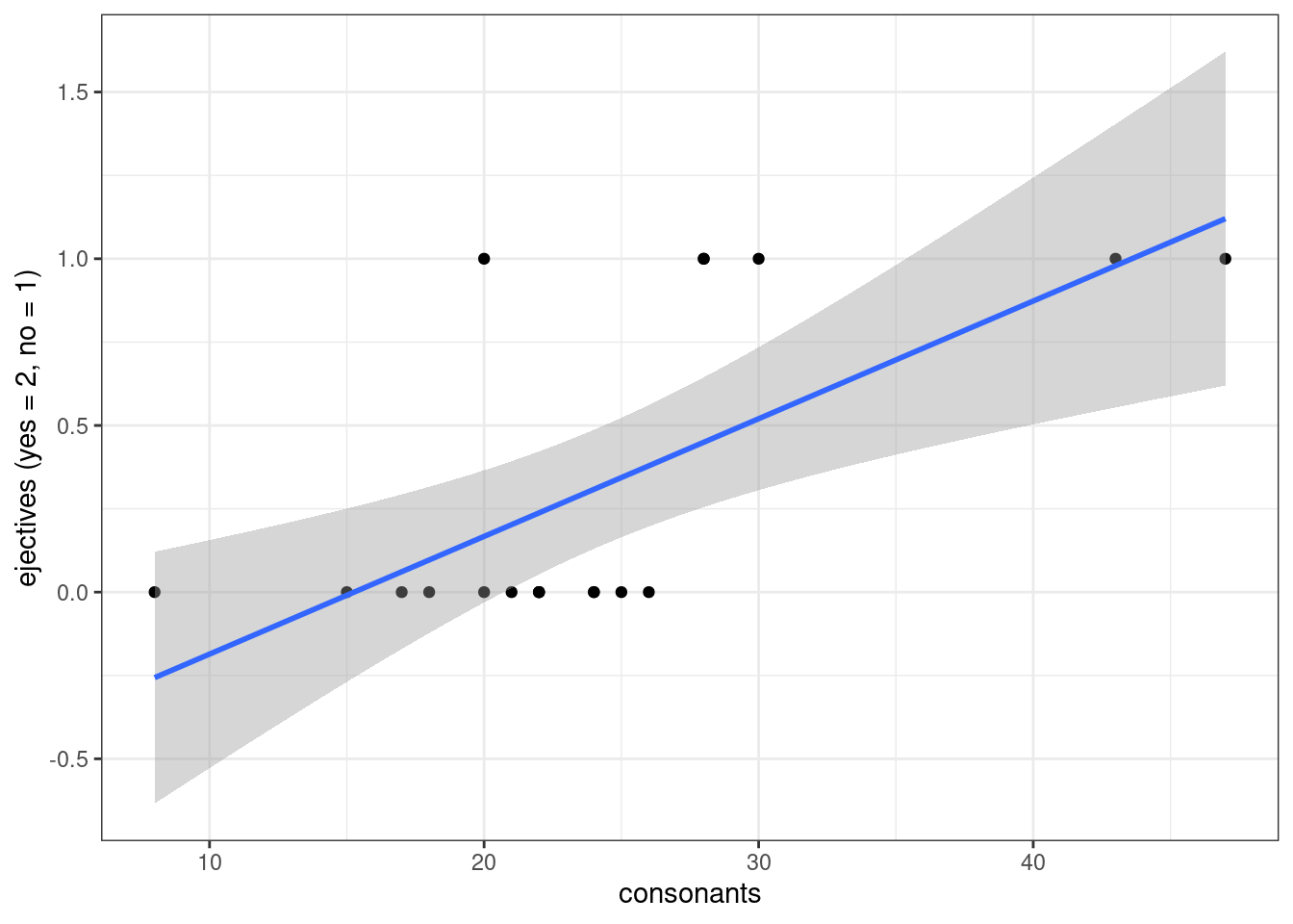
10.1.2.2 Модель без предиктора
logit_0 <- glm(ejectives~1, family = "binomial", data = phonological_profiles)
summary(logit_0)
Call:
glm(formula = ejectives ~ 1, family = "binomial", data = phonological_profiles)

Deviance Residuals:
    Min       1Q   Median       3Q      Max
-0.8712  -0.8712  -0.8712   1.5183   1.5183

Coefficients:
            Estimate Std. Error z value Pr(>|z|)
(Intercept)  -0.7732     0.4935  -1.567    0.117

(Dispersion parameter for binomial family taken to be 1)

    Null deviance: 23.699  on 18  degrees of freedom
Residual deviance: 23.699  on 18  degrees of freedom
AIC: 25.699

Number of Fisher Scoring iterations: 4logit_0$coefficients(Intercept)
-0.7731899 table(phonological_profiles$ejectives)
FALSE  TRUE
13 6 log(6/13) # β0[1] -0.77318996/(13+6) # p[1] 0.3157895exp(log(6/13))/(1+exp(log(6/13))) # p[1] 0.3157895Какой коэфициент логистической регрессии, мы получим, запустив модель, предсказывающую количество s-генитивов, если наши данные состоят из 620 s-генитивов из 699 генетивных контекстов?
Ответ округлите до трех и меньше знаков после запятой.
10.1.2.3 Модель c одним числовым предиктором
logit_1 <- glm(ejectives~consonants, family = "binomial", data = phonological_profiles)
summary(logit_1)
Call:
glm(formula = ejectives ~ consonants, family = "binomial", data = phonological_profiles)

Deviance Residuals:
     Min        1Q    Median        3Q       Max
-1.08779  -0.49331  -0.20265   0.02254   2.45384

Coefficients:
            Estimate Std. Error z value Pr(>|z|)
(Intercept) -12.1123     6.1266  -1.977   0.0480 *
consonants    0.4576     0.2436   1.878   0.0603 .
---
Signif. codes:  0 '***' 0.001 '**' 0.01 '*' 0.05 '.' 0.1 ' ' 1

(Dispersion parameter for binomial family taken to be 1)

    Null deviance: 23.699  on 18  degrees of freedom
Residual deviance: 12.192  on 17  degrees of freedom
AIC: 16.192

Number of Fisher Scoring iterations: 6logit_1$coefficients(Intercept) consonants
-12.1123347 0.4576095 phonological_profiles %>%
mutate(ejectives = as.double(ejectives)) %>%
ggplot(aes(consonants, ejectives)) +
geom_smooth(method = "glm",
method.args = list(family = "binomial"),
se = FALSE)+
geom_point()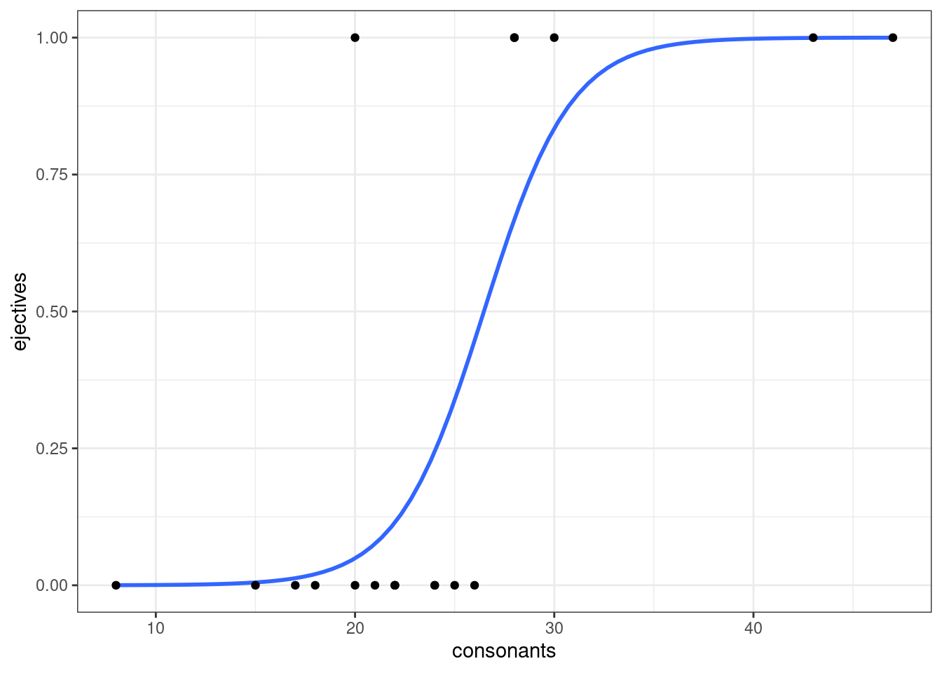
Какова вероятность, что в языке с 29 согласными есть абруптивные?
logit_1$coefficients(Intercept) consonants
-12.1123347 0.4576095 \[\log\left({\frac{p}{1-p}}\right)_i=\beta_0+\beta_1\times consinants_i + \epsilon_i\] \[\log\left({\frac{p}{1-p}}\right)=-12.1123347 + 0.4576095 \times 29 = 1.158341\] \[p = \frac{e^{1.158341}}{1+e^{1.158341}} = 0.7610311\]
# log(odds)
predict(logit_1, newdata = data.frame(consonants = 29))
1
1.158341 # p
predict(logit_1, newdata = data.frame(consonants = 29), type = "response") 1
0.7610312 Какой логорифм шансов предсказывает наша модель для языка с 25 согласными (6 знаков после запятой)?
Какую вероятность предсказывает наша модель для языка с 25 согласными (6 знаков после запятой)?
10.1.2.4 Модель c одним категориальным предиктором
logit_2 <- glm(ejectives~area, family = "binomial", data = phonological_profiles)
summary(logit_2)
Call:
glm(formula = ejectives ~ area, family = "binomial", data = phonological_profiles)

Deviance Residuals:
     Min        1Q    Median        3Q       Max
-1.66511  -0.55525  -0.00013   0.75853   1.97277

Coefficients:
                                  Estimate               Std. Error z value
(Intercept)         -0.0000000000000001245    0.9999999999999997780   0.000
areaAustralia      -18.5660685098658397862 6522.6386791247941800975  -0.003
areaEurasia         -1.7917594692280540691    1.4719601443879741787  -1.217
areaNorth America    1.0986122886681095601    1.5275252316519460916   0.719
areaPapunesia      -18.5660685098631610401 6522.6386791219219958293  -0.003
areaSouth America  -18.5660685098637685542 4612.2020954414929292398  -0.004
                  Pr(>|z|)
(Intercept)          1.000
areaAustralia        0.998
areaEurasia          0.224
areaNorth America    0.472
areaPapunesia        0.998
areaSouth America    0.997

(Dispersion parameter for binomial family taken to be 1)

    Null deviance: 23.699  on 18  degrees of freedom
Residual deviance: 15.785  on 13  degrees of freedom
AIC: 27.785

Number of Fisher Scoring iterations: 17logit_2$coefficients (Intercept) areaAustralia areaEurasia
-0.000000000000000124505 -18.566068509865839786244 -1.791759469228054069134
areaNorth America areaPapunesia areaSouth America
1.098612288668109560064 -18.566068509863161040130 -18.566068509863768554169 table(phonological_profiles$ejectives, phonological_profiles$area)
        Africa Australia Eurasia North America Papunesia South America
  FALSE      2         1       6             1         1             2
TRUE 2 0 1 3 0 0log(1/6) # Eurasia[1] -1.791759log(3/1) # North America[1] 1.09861210.1.2.5 Множественная регрессия
logit_3 <- glm(ejectives~consonants+area, family = "binomial", data = phonological_profiles)
summary(logit_3)
Call:
glm(formula = ejectives ~ consonants + area, family = "binomial",
    data = phonological_profiles)

Deviance Residuals:
     Min        1Q    Median        3Q       Max
-1.54011  -0.18623  -0.00012   0.00023   1.53307

Coefficients:
                    Estimate Std. Error z value Pr(>|z|)
(Intercept)         -21.1760    15.1089  -1.402    0.161
consonants            0.8137     0.5653   1.439    0.150
areaAustralia       -16.2910 10754.0138  -0.002    0.999
areaEurasia          -1.2069     3.9399  -0.306    0.759
areaNorth America     4.0966     4.8563   0.844    0.399
areaPapunesia        -4.8995 10754.0184   0.000    1.000
areaSouth America   -17.1162  7065.6839  -0.002    0.998

(Dispersion parameter for binomial family taken to be 1)

    Null deviance: 23.6989  on 18  degrees of freedom
Residual deviance:  6.7901  on 12  degrees of freedom
AIC: 20.79

Number of Fisher Scoring iterations: 18
10.1.2.6 Cравнение моделей
AIC(logit_0, logit_1, logit_2, logit_3)BIC(logit_0, logit_1, logit_2, logit_3)Выберите наилучшую модель согласно AIC и BIC:
Для того, чтобы интерпретировать коэффициенты нужно проделать трансформацию:
(exp(logit_1$coefficients)-1)*100(Intercept) consonants
-99.99945 58.02918 Перед нами процентное изменние шансов при увеличении независимой переменной на 1.
Было предложено много аналогов R\(^2\), например, McFadden’s R squared:
pscl::pR2(logit_1)fitting null model for pseudo-r2 llh llhNull G2 McFadden r2ML r2CU
-6.0958355 -11.8494421 11.5072132 0.4855593 0.4542765 0.6373812 Проанализируйте в датасете с языками связь количества сегментов и наличия ударения. Постройте регрессию, визуализируйте связь. Какой вывод вы можете сделать?
10.2 Порядковая логистическая регрессия
Данные взяты из исследования [Endresen, Janda 2015], посвященное исследованию маргинальных глаголов изменения состояния в русском языке. Испытуемые (70 школьников, 51 взрослый) оценивали по шкале Ликерта (1…5) приемлемость глаголов с приставками о- и у-:
- широко используемуе в СРЛЯ (освежить, уточнить)
- встретившие всего несколько раз в корпусе (оржавить, увкуснить)
- искусственные слова (ономить, укампить)
marginal_verbs <- read_csv("https://raw.githubusercontent.com/agricolamz/2021_da4l/master/data/marginal_verbs.csv")
head(marginal_verbs)
Переменные в датасете:
- Gender
- Age
- AgeGroup — взрослые или школьники
- Education
- City
- SubjectCode — код испытуемого
- Score — оценка, поставленная испытуемым (A — самая высокая, E — самая низкая)
- GivenScore — оценка, поставленная испытуемым (5 — самая высокая, 1 — самая низкая)
- Stimulus
- Prefix
- WordType — тип слова: частотное, редкое, искусственное
- CorpusFrequency — частотность в корпусе
marginal_verbs$Score <- factor(marginal_verbs$Score)
levels(marginal_verbs$Score)
[1] "A" "B" "C" "D" "E"ordinal <- MASS::polr(Score~Prefix+WordType+CorpusFrequency, data = marginal_verbs)
summary(ordinal)Call:
MASS::polr(formula = Score ~ Prefix + WordType + CorpusFrequency,
data = marginal_verbs)
Coefficients:
Value Std. Error t value
Prefixu 0.136619 0.05286365 2.584
WordTypenonce 1.340603 0.05692826 23.549
WordTypestandard -4.655327 0.12510542 -37.211
CorpusFrequency -0.001015 0.00007879 -12.876
Intercepts:
Value Std. Error t value
A|B -2.6275 0.0753 -34.8784
B|C -1.4531 0.0552 -26.3246
C|D -0.2340 0.0479 -4.8853
D|E 0.7324 0.0492 14.8986
Residual Deviance: 13138.47
AIC: 13154.47 ordinal$coefficients Prefixu WordTypenonce WordTypestandard CorpusFrequency
0.136619412 1.340602696 -4.655327418 -0.001014583 Как и раньше, можно преобразовать коэффициенты:
(exp(ordinal$coefficients)-1)*100 Prefixu WordTypenonce WordTypestandard CorpusFrequency
14.6391763 282.1345921 -99.0489201 -0.1014068 \[\log(\frac{p(A)}{p(B|C|D|E)}) = -2.6275 + 0.136619412 \times Prefixu +\]
\[+ 1.340602696 \times WordTypenonce -\]
\[-4.655327418 \times WordTypestandard - \]
\[ - 0.001014583\times CorpusFrequency\]
\[\log(\frac{p(A|B)}{p(C|D|E)}) = -1.4531 + 0.136619412 \times Prefixu + \]
\[ + 1.340602696 \times WordTypenonce-\]
\[-4.655327418 \times WordTypestandard -\]
\[ -0.001014583\times CorpusFrequency\]
\[\log(\frac{p(A|B|C)}{p(D|E)}) = -0.2340 + 0.136619412 \times Prefixu + \]
\[ + 1.340602696 \times WordTypenonce-\]
\[-4.655327418 \times WordTypestandard - \]
\[-0.001014583\times CorpusFrequency\]
\[\log(\frac{p(A|B|C|D)}{p(E)}) = 0.7324 + 0.136619412 \times Prefixu +\] \[ + 1.340602696 \times WordTypenonce-\] \[-4.655327418 \times WordTypestandard -\] \[=0.001014583\times CorpusFrequency\]
head(predict(ordinal))[1] A A E E A A
Levels: A B C D Ehead(predict(ordinal, type = "probs")) A B C D E
1 0.99178000 0.005665533 0.001798242 0.0004683707 0.0002878525
2 0.93841926 0.041706786 0.013917668 0.0036817261 0.0022745617
3 0.06764594 0.122509282 0.252611927 0.2334448870 0.3237879649
4 0.01855865 0.039108932 0.113894002 0.1808984667 0.6475399508
5 0.90986002 0.060436871 0.020738032 0.0055351143 0.0034299624
6 0.91496678 0.057117954 0.019500629 0.0051963745 0.0032182669marginal_verbs %>%
bind_cols(as_tibble(predict(ordinal, type = "probs"))) %>%
gather(score, predictions, A:E) %>%
ggplot(aes(x = score, y = predictions, fill = score)) +
geom_col(position = "dodge")+
facet_grid(Prefix~WordType)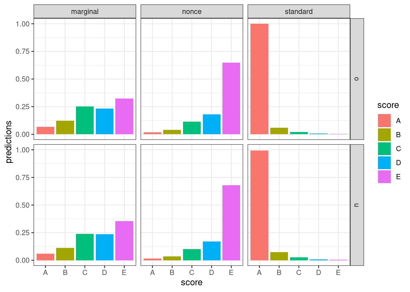
library(ggeffects)
ordinal %>%
  ggpredict(terms = c("Prefix", "WordType")) %>%
  plot()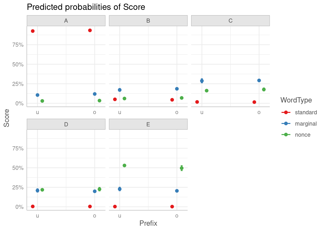
10.3 Мультиномиальная регрессия
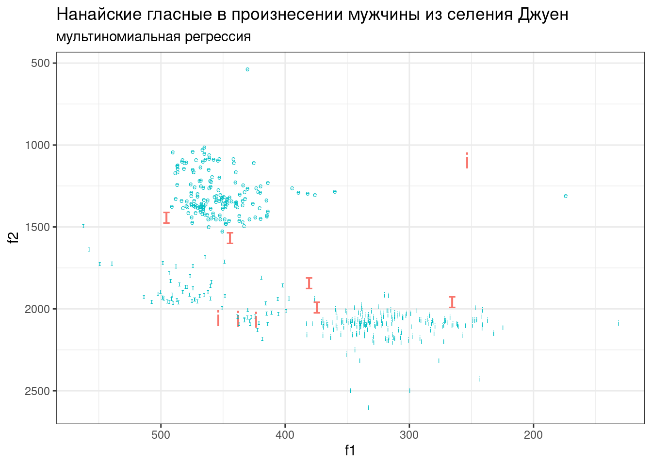
В этом датасете представлены три нанайских гласных i, ɪ и e, произнесенные нанайским носителем мужского пола из селения Джуен. Каждая строчка — отдельное произнесение. Переменные:
- f1 — первая форманта
- f2 — вторая форманта
nanai <- read_csv("https://raw.githubusercontent.com/agricolamz/2021_da4l/master/data/nanai_vowels.csv")
nanai %>%
  ggplot(aes(f2, f1, label = sound, color = sound))+
  geom_text()+
  geom_rug()+
  scale_y_reverse()+
  scale_x_reverse()+
  stat_ellipse()+
  theme_bw()+
  theme(legend.position = "none")+
  labs(title = "Нанайские гласные в произнесении мужчины из селения Джуен")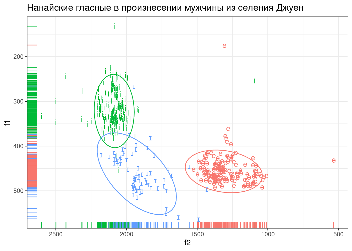
mult <- nnet::multinom(sound~f1+f2, data = nanai)# weights: 12 (6 variable)
initial value 462.515774
iter 10 value 51.522626
iter 20 value 46.817442
iter 30 value 44.829080
iter 40 value 44.807654
iter 40 value 44.807654
final value 44.807654
convergedmultCall:
nnet::multinom(formula = sound ~ f1 + f2, data = nanai)
Coefficients:
(Intercept) f1 f2
i -22.85202 -0.04263175 0.02315226
ɪ -41.46147 0.02360077 0.01937067
Residual Deviance: 89.61531
AIC: 101.6153 \[\log(\frac{p(e)}{p(ɪ)}) = -41.46147 + 0.02360077\times f1 +0.01937067\times f2\] \[\log(\frac{p(i)}{p(ɪ)}) = -22.85202 -0.04263175\times f1 + 0.02315226\times f2\]
nanai %>%
  mutate(prediction = predict(mult),
         correctness = sound == prediction) %>%
  ggplot(aes(f1, f2, label = sound, color = correctness))+
  geom_text(aes(size = !correctness), show.legend = FALSE)+
  scale_y_reverse()+
  scale_x_reverse()+
  theme_bw()+
  labs(title = "Нанайские гласные в произнесении мужчины из селения Джуен",
       subtitle = "мультиномиальная регрессия")