Корреляция и регрессия

Correlation

library(tidyverse)
cor(mtcars$mpg,mtcars$qsec)

## [1] 0.418684

a <- cor.test(mtcars$mpg,mtcars$qsec)
a$conf.int

## [1] 0.08195487 0.66961864
## attr(,"conf.level")
## [1] 0.95

mtcars %>% 
  cor()

##             mpg        cyl       disp         hp        drat         wt
## mpg   1.0000000 -0.8521620 -0.8475514 -0.7761684  0.68117191 -0.8676594
## cyl  -0.8521620  1.0000000  0.9020329  0.8324475 -0.69993811  0.7824958
## disp -0.8475514  0.9020329  1.0000000  0.7909486 -0.71021393  0.8879799
## hp   -0.7761684  0.8324475  0.7909486  1.0000000 -0.44875912  0.6587479
## drat  0.6811719 -0.6999381 -0.7102139 -0.4487591  1.00000000 -0.7124406
## wt   -0.8676594  0.7824958  0.8879799  0.6587479 -0.71244065  1.0000000
## qsec  0.4186840 -0.5912421 -0.4336979 -0.7082234  0.09120476 -0.1747159
## vs    0.6640389 -0.8108118 -0.7104159 -0.7230967  0.44027846 -0.5549157
## am    0.5998324 -0.5226070 -0.5912270 -0.2432043  0.71271113 -0.6924953
## gear  0.4802848 -0.4926866 -0.5555692 -0.1257043  0.69961013 -0.5832870
## carb -0.5509251  0.5269883  0.3949769  0.7498125 -0.09078980  0.4276059
##             qsec         vs          am       gear        carb
## mpg   0.41868403  0.6640389  0.59983243  0.4802848 -0.55092507
## cyl  -0.59124207 -0.8108118 -0.52260705 -0.4926866  0.52698829
## disp -0.43369788 -0.7104159 -0.59122704 -0.5555692  0.39497686
## hp   -0.70822339 -0.7230967 -0.24320426 -0.1257043  0.74981247
## drat  0.09120476  0.4402785  0.71271113  0.6996101 -0.09078980
## wt   -0.17471588 -0.5549157 -0.69249526 -0.5832870  0.42760594
## qsec  1.00000000  0.7445354 -0.22986086 -0.2126822 -0.65624923
## vs    0.74453544  1.0000000  0.16834512  0.2060233 -0.56960714
## am   -0.22986086  0.1683451  1.00000000  0.7940588  0.05753435
## gear -0.21268223  0.2060233  0.79405876  1.0000000  0.27407284
## carb -0.65624923 -0.5696071  0.05753435  0.2740728  1.00000000

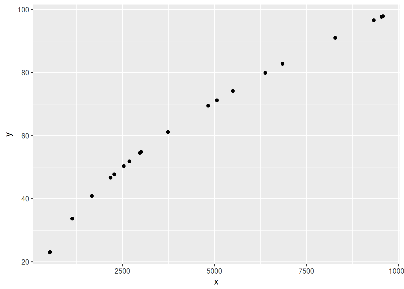
df <- data.frame(y = runif(20, 20, 100))
df %>% 
  mutate(x = y^2) %>%
  cor(method = "p")

##           y         x
## y 1.0000000 0.9837302
## x 0.9837302 1.0000000

df %>% 
  mutate(x = y^2) %>%
  ggplot(aes(x, y)) +
  geom_point()

number = 
dat <- read.csv("https://goo.gl/5bp7hH")
dat %>% 
  group_by(s.deletion) %>% 
  summarize(number = n())

## # A tibble: 2 × 2
##   s.deletion number
##       <fctr>  <int>
## 1         no   3755
## 2        yes   5091

dat %>% 
  group_by(s.deletion, gramm.cat, phon.cont) %>% 
  summarize(number = n())

## Source: local data frame [26 x 4]
## Groups: s.deletion, gramm.cat [?]
## 
##    s.deletion         gramm.cat phon.cont number
##        <fctr>            <fctr>    <fctr>  <int>
## 1          no         adjective consonant    261
## 2          no         adjective     pause     22
## 3          no         adjective     vowel     28
## 4          no        determiner consonant    678
## 5          no        determiner     vowel    111
## 6          no              noun consonant    418
## 7          no              noun     pause    132
## 8          no              noun     vowel    124
## 9          no separate morpheme consonant   1361
## 10         no separate morpheme     pause    146
## # ... with 16 more rows