3 Data manipulation: `dplyr`

First, load the library:

library(tidyverse)

3.1 Data

In this chapter we will use the following datasets.

3.1.1 Misspelling dataset

I gathered this dataset after some manipulations with data from The Gyllenhaal Experiment by Russell Goldenberg and Matt Daniels for pudding. They analized mistakes in spellings of celebrities during the searching process.

misspellings <- read_csv("https://raw.githubusercontent.com/agricolamz/2020.02_Naumburg_R/master/data/misspelling_dataset.csv")

## Parsed with column specification:
## cols(
##   correct = col_character(),
##   spelling = col_character(),
##   count = col_double()
## )

misspellings

There are the following variables in this dataset:

correct — correct spelling
spelling — user’s spelling
count — number of cases of user’s spelling

3.1.2 `diamonds`

diamonds — is the dataset built-in in the tidyverse package.

diamonds

?diamonds

3.2 `dplyr`

Here and here is a cheatsheet on dplyr.

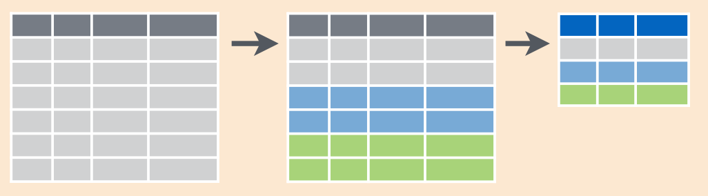
3.2.1 `filter()`

This function filters rows under some conditions.

How many wrong spellings were used by less then 10 users?

misspellings %>%
  filter(count < 10)

%>% it is pipe (hot key is Ctrl Shift M). It allows to chain operations, putting the output of one function into the input of another:

sort(sqrt(abs(sin(1:22))), decreasing = TRUE)

##  [1] 0.9999951 0.9952926 0.9946649 0.9805088 0.9792468 0.9554817 0.9535709
##  [8] 0.9173173 0.9146888 0.8699440 0.8665952 0.8105471 0.8064043 0.7375779
## [15] 0.7325114 0.6482029 0.6419646 0.5365662 0.5285977 0.3871398 0.3756594
## [22] 0.0940814

1:22 %>% 
  sin() %>% 
  abs() %>% 
  sqrt() %>% 
  sort(., decreasing = TRUE) # why do we need a dot here?

##  [1] 0.9999951 0.9952926 0.9946649 0.9805088 0.9792468 0.9554817 0.9535709
##  [8] 0.9173173 0.9146888 0.8699440 0.8665952 0.8105471 0.8064043 0.7375779
## [15] 0.7325114 0.6482029 0.6419646 0.5365662 0.5285977 0.3871398 0.3756594
## [22] 0.0940814

Pipes that are used in tidyverse are from the package magrittr. Sometimes pipe could work not well with functions outside the tidyverse.

So filter() function returns rows with matching conditions:

misspellings %>%
  filter(count < 10)

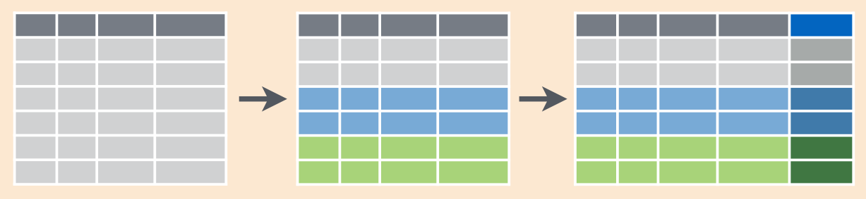
It is possible to use multiple conditions. How many wrong spellings of Deschanel were used by less then 10 users?

misspellings %>%
  filter(count < 10,
         correct == "deschanel")

It is possible to use OR conditions. How many wrong spellings were used by less then 10 OR more then 500 users?

misspellings %>%
  filter(count < 10 |
           count > 500)

3.2.2 `slice()`

This function filters rows by its index.

misspellings %>%
  slice(3:7)

3.2.3 `select()`

This functions for choosing variables from a dataframe.

diamonds %>%
  select(8:10)

diamonds %>%
  select(color:price)

diamonds %>%
  select(-carat)

diamonds %>%
  select(-c(carat, cut, x, y, z))

diamonds %>%
  select(cut, depth, price)

3.2.4 `arrange()`

This function orders rows in a dataframe (numbers — by order, strings — alphabetically).

misspellings %>%
  arrange(count)

diamonds %>%
  arrange(desc(carat), price)

diamonds %>%
  arrange(-carat, price)

3.2.5 `distinct()`

This function returns only unique rows from an input dataframe.

misspellings %>%
  distinct(correct)

misspellings %>%
  distinct(spelling)

diamonds %>%
  distinct(color, cut)

In built-in dataset starwars filter those characters that are higher then 180 (height) and weigh less then 80 (mass). How many unique names of their homeworlds (homeworld) is there?

3.2.6 `mutate()`

This function creates new variables.

misspellings %>%
  mutate(misspelling_length = nchar(spelling),
         id = 1:n())

Create a variable with body mass index Body mass index: \(\frac{mass}{height^2}\) for all characters from starwars dataset. How many charachters have obesity (have body mass index greater 30)? (Don’t forget to convert height from centimetres to metres).

3.2.7 `group_by(...) %>% summarise(...)`

This function allows to group variables by some columns and get some descriptive statistics (maximum, minimum, last value, first value, mean, median etc.)

misspellings %>%
  summarise(min(count), mean(count))

misspellings %>%
  group_by(correct) %>% 
  summarise(mean(count))

misspellings %>%
  group_by(correct) %>% 
  summarise(my_mean = mean(count))

If you need to calculate number of cases, use the function n() in summarise() or the count() function:

misspellings %>%
  group_by(correct) %>% 
  summarise(n = n())

misspellings %>%
  count(correct)

It is even possible to sort the result, using sort argument:

misspellings %>%
  count(correct, sort = TRUE)

In case you don’t want to have any summary, but an additional column, just replace summarise() with mutate()

misspellings %>%
  group_by(correct) %>% 
  mutate(my_mean = mean(count))

Here is a scheme:

In the starwars dataset create a variable that contains mean height value for each species.

3.3 Merging dataframes

3.3.1 `bind_...`

This is a family of functions that make it possible to merge dataframes together:

my_tbl <- tibble(a  = c(1, 5, 2), 
                 b = c("e", "g", "s"))

Here is how to merge two datasets by row:

my_tbl %>% 
  bind_rows(my_tbl)

In case there is an absent column, values will be filled with NA:

my_tbl %>% 
  bind_rows(my_tbl[,-1])

In order to merge dataframes by column you need another function:

my_tbl %>% 
  bind_cols(my_tbl)

In case there is an absent row, this function will return an error:

my_tbl %>% 
  bind_cols(my_tbl[-1,])

## Error: Argument 2 must be length 3, not 2

3.3.2 `.._join()`

These functions allow to merge different datasets by some column (or columns in common).

languages <- data_frame(
  languages = c("Selkup", "French", "Chukchi", "Polish"),
  countries = c("Russia", "France", "Russia", "Poland"),
  iso = c("sel", "fra", "ckt", "pol")
  )

## Warning: `data_frame()` is deprecated, use `tibble()`.
## This warning is displayed once per session.

languages

country_population <- data_frame(
  countries = c("Russia", "Poland", "Finland"),
  population_mln = c(143, 38, 5))
country_population

inner_join(languages, country_population)

## Joining, by = "countries"

left_join(languages, country_population)

## Joining, by = "countries"

right_join(languages, country_population)

## Joining, by = "countries"

anti_join(languages, country_population)

## Joining, by = "countries"

anti_join(country_population, languages)

## Joining, by = "countries"

full_join(country_population, languages)

## Joining, by = "countries"

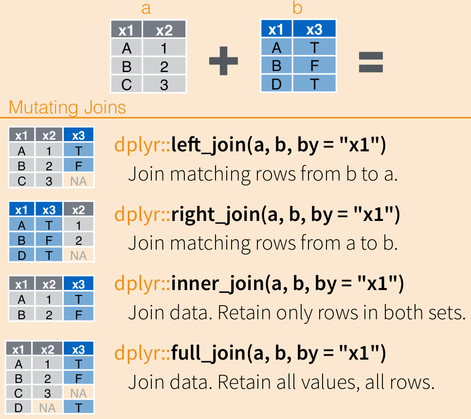
3.4 `tidyr` package

Here is a dataset with the number of speakers of some language of India according the census 2001 (data from Wikipedia):

langs_in_india_short <- read_csv("https://raw.githubusercontent.com/agricolamz/2020.02_Naumburg_R/master/data/languages_in_india.csv")

## Parsed with column specification:
## cols(
##   language = col_character(),
##   n_L1_sp = col_double(),
##   n_L2_sp = col_double(),
##   n_L3_sp = col_double(),
##   n_all_sp = col_double()
## )

Wide format

langs_in_india_short

Long format

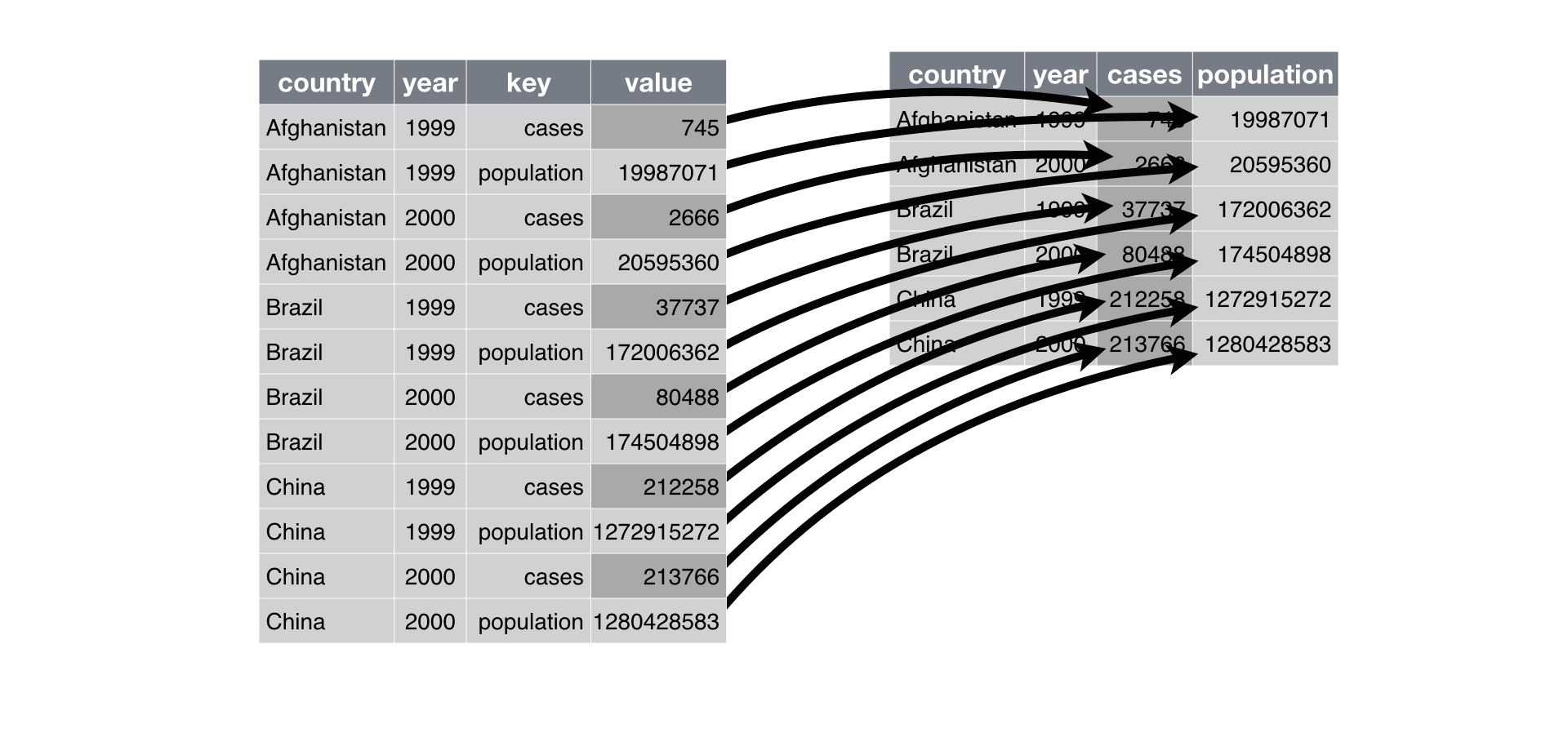
Wide format → Long format: tidyr::pivot_longer()

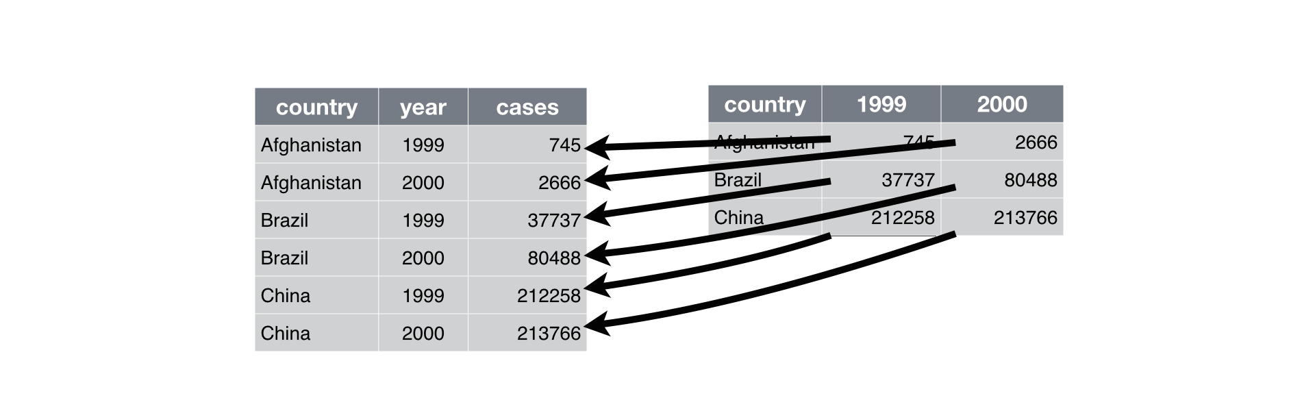
langs_in_india_short %>% 
  pivot_longer(names_to = "type", values_to = "n_speakers", n_L1_sp:n_all_sp)->
  langs_in_india_long

langs_in_india_long

Long format → Wide format: tidyr::pivot_wider()

langs_in_india_long %>% 
  pivot_wider(names_from = "type", values_from = "n_speakers")->
  langs_in_india_short
langs_in_india_short

3.4.1 Tidy data

You can represent the same underlying data in multiple ways. The whole tidyverse phylosophy built upon the tidy datasets, that are datasets where:

Each variable must have its own column.
Each observation must have its own row.
Each value must have its own cell.

Here is data, that contains information about villages of Daghestan in .xlsx format. The data is separated by different sheets and contains the following variables (data obtained from different sources, so they have suffixes _s1 – first source and _s2 – second source):

id_s1 – (s1) identification number from first source;
name_1885 – (s1) name of the village according the 1885 census
census_1885 – (s1) population according the 1885 census
name_1895 – (s1) name of the village according the 1895 census
census_1895 – (s1) population according the 1895 census
name_1926 – (s1) name of the village according the 1926 census
census_1926 – (s1) population according the 1926 census
name_2010 – (s1) name of the village according the 2010 census
census_2010 – (s1) population according the 2010 census
language_s1 – (s1) language name according the first source
name_s2 – (s2) village name according the second source
language_s2 – (s2) language name according the second source
Lat – (s2) latitude
Lon – (s2) longitude
elevation – (s2) altitude

First, merge all sheets fromt the .xlsx file:

Second, caclulate how many times the language name is the same in both sources.

Third, calculate mean altitude for languages from the first source. Which is the highest?

Fourth, calculate the population for languages from the second source in each census. Show the values obtained for the Lak language:

3 Data manipulation: dplyr

3.1 Data

3.1.1 Misspelling dataset

3.1.2 diamonds

3.2 dplyr

3.2.1 filter()

3.2.2 slice()

3.2.3 select()

3.2.4 arrange()

3.2.5 distinct()

3.2.6 mutate()

3.2.7 group_by(...) %>% summarise(...)