6 Text manipulations
I will still use a lot of tidyverse:
6.1 read_lines()
If you want to read text in R you can use the read_lines() function:
tajemnica_baskerville <- read_lines("https://raw.githubusercontent.com/agricolamz/2020.02_Naumburg_R/master/data/tajemnica_baskerville.txt")As a result you will get a vector with characters. It is easy to convert it to dataframe:
6.2 gutenbergr
The gutenbergr package is an API for a very old project Gutenberg, that is a library of over 60,000 free eBooks.
The most important part of this package is the gutenberg_metadata dataset – that is a catalogue of everything in the Gutenberg library.
## Classes 'tbl_df', 'tbl' and 'data.frame': 51997 obs. of 8 variables:
## $ gutenberg_id : int 0 1 2 3 4 5 6 7 8 9 ...
## $ title : chr NA "The Declaration of Independence of the United States of America" "The United States Bill of Rights\r\nThe Ten Original Amendments to the Constitution of the United States" "John F. Kennedy's Inaugural Address" ...
## $ author : chr NA "Jefferson, Thomas" "United States" "Kennedy, John F. (John Fitzgerald)" ...
## $ gutenberg_author_id: int NA 1638 1 1666 3 1 4 NA 3 3 ...
## $ language : chr "en" "en" "en" "en" ...
## $ gutenberg_bookshelf: chr NA "United States Law/American Revolutionary War/Politics" "American Revolutionary War/Politics/United States Law" NA ...
## $ rights : chr "Public domain in the USA." "Public domain in the USA." "Public domain in the USA." "Public domain in the USA." ...
## $ has_text : logi TRUE TRUE TRUE TRUE TRUE TRUE ...
## - attr(*, "date_updated")= Date, format: "2016-05-05"How many languages are presented in the Gutenberg library?
How many authors are available?
How many Polish texts are available?
Whose texts are the most numerous in the German part of the Gutenberg library? Put his/her last name in the form.
Let’s have a look at Mickiewicz’s texts in the Polish part of the Gutenberg library:
Let’s download Adam Mickiewicz’s sonnets:
It is possible to use multiple ids. Let’s also download some poems by A. Mickiewicz (1798–1855), J. Kochanowski (1530–1584), Z. Krasinski (1812–1859), and A. Oppman (1867–1931):
Be aware:
- texts could include something from the real book: introduction or last word written by other people, publication details, etc.
- texts could be stored with the wrong encoding;
- texts could be stored with normalised orthography (e. g. Kochanowski, look at rows 99 and 100);
- there are a lot of empty characters;
- and probably a lot of other problems.
I annotated those texts:
texts <- read_csv("https://raw.githubusercontent.com/agricolamz/2020.02_Naumburg_R/master/data/mickiewicz_kochanowski_krasinski_oppman.csv")Now it is possible to remove some non-important lines:
Calculate how many rows per author we do have in our dataset. Who has the largest amount?
6.3 tidytext
The tidytext (Silge and Robinson 2017) (this book is available online) allows you to work with texts in tidy ideology, that makes it easier to manipulate, summarise, and visualise the characteristics of texts easily and integrate natural language processing tools (sentiment analysis, tf-idf metric, n-gram analysis, topic modeling etc.).
texts %>%
unnest_tokens(output = "word", input = text) %>%
group_by(author) %>%
count(word, sort = TRUE) %>%
top_n(10) %>%
ggplot(aes(word, n))+
geom_col()+
coord_flip()+
facet_wrap(~author, scales = "free")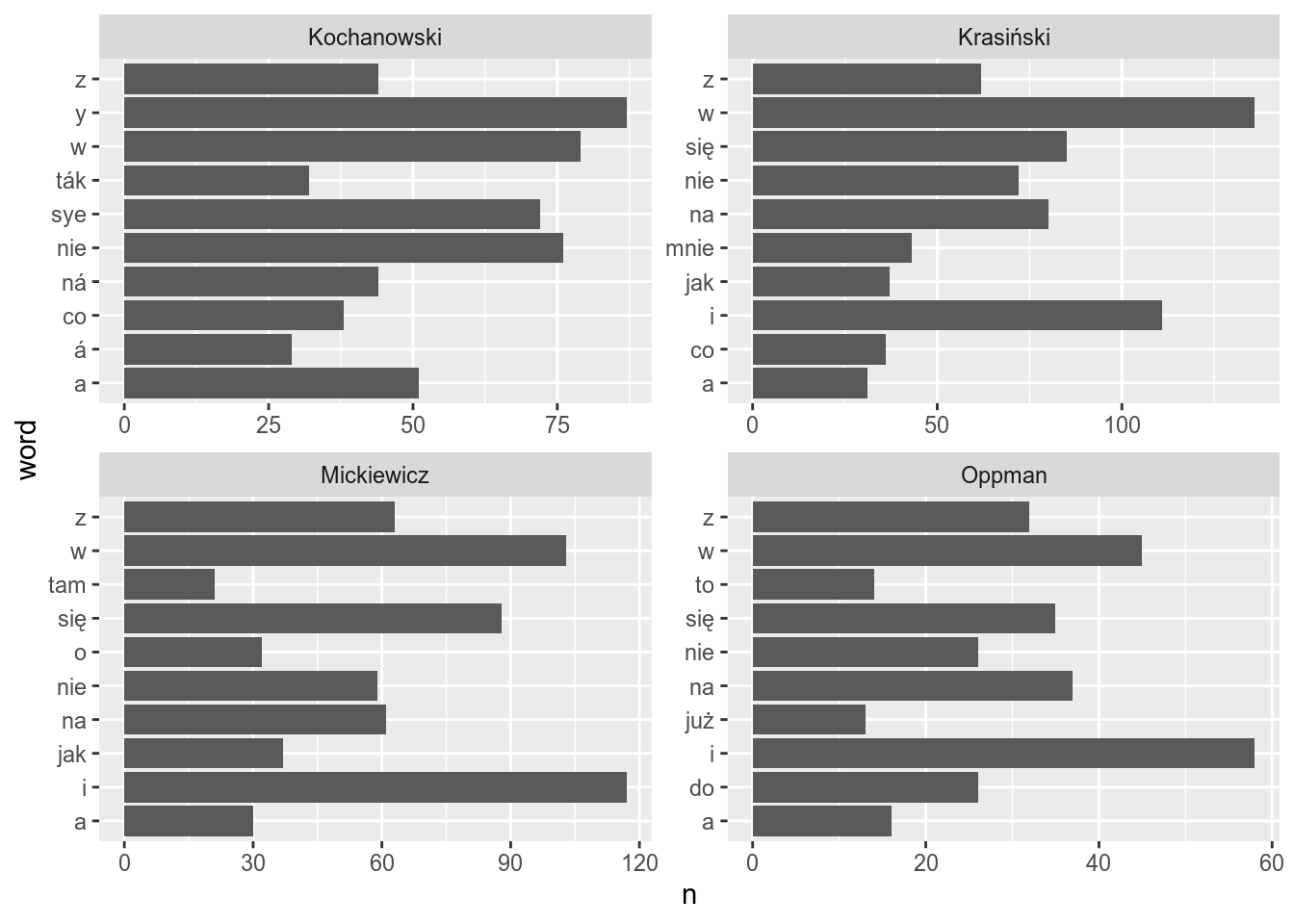
As you see the sorting is bad. Sorting within different facets is possible with the reorder_within() function:
texts %>%
unnest_tokens(output = "word", input = text) %>%
group_by(author) %>%
count(word, sort = TRUE) %>%
top_n(10) %>%
ggplot(aes(reorder_within(x = word, by = n, within = author), n))+
geom_col()+
coord_flip()+
facet_wrap(~author, scales = "free")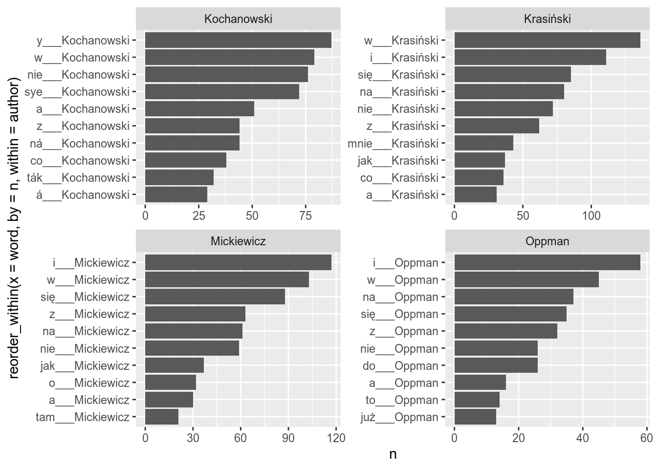
In order to remove the authors name you also need to add scale_x_reordered() layer to your ggplot:
texts %>%
unnest_tokens(output = "word", input = text) %>%
group_by(author) %>%
count(word, sort = TRUE) %>%
top_n(10) %>%
ggplot(aes(reorder_within(word, n, author), n))+
geom_col()+
scale_x_reordered()+
coord_flip()+
facet_wrap(~author, scales = "free")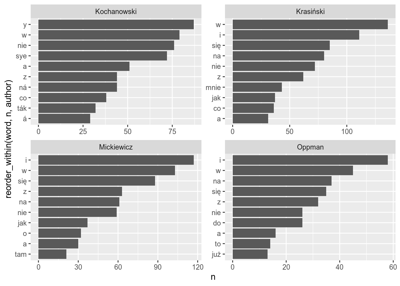
Often in text analysis, it is useful to remove stopwords. Stop words are frequent words that mostly contain grammatic information. I will use a polish stopword-list from this repository, but you can use any other list or modify the existing one.
stopwords <- read_lines("https://raw.githubusercontent.com/stopwords-iso/stopwords-pl/master/stopwords-pl.txt")
stopwords## [1] "a" "aby" "ach" "acz" "aczkolwiek"
## [6] "aj" "albo" "ale" "ależ" "ani"
## [11] "aż" "bardziej" "bardzo" "bez" "bo"
## [16] "bowiem" "by" "byli" "bym" "bynajmniej"
## [21] "być" "był" "była" "było" "były"
## [26] "będzie" "będą" "cali" "cała" "cały"
## [31] "chce" "choć" "ci" "ciebie" "cię"
## [36] "co" "cokolwiek" "coraz" "coś" "czasami"
## [41] "czasem" "czemu" "czy" "czyli" "często"
## [46] "daleko" "dla" "dlaczego" "dlatego" "do"
## [51] "dobrze" "dokąd" "dość" "dr" "dużo"
## [56] "dwa" "dwaj" "dwie" "dwoje" "dzisiaj"
## [61] "dziś" "gdy" "gdyby" "gdyż" "gdzie"
## [66] "gdziekolwiek" "gdzieś" "go" "godz" "hab"
## [71] "i" "ich" "ii" "iii" "ile"
## [76] "im" "inna" "inne" "inny" "innych"
## [81] "inż" "iv" "ix" "iż" "ja"
## [86] "jak" "jakaś" "jakby" "jaki" "jakichś"
## [91] "jakie" "jakiś" "jakiż" "jakkolwiek" "jako"
## [96] "jakoś" "je" "jeden" "jedna" "jednak"
## [101] "jednakże" "jedno" "jednym" "jedynie" "jego"
## [106] "jej" "jemu" "jest" "jestem" "jeszcze"
## [111] "jeśli" "jeżeli" "już" "ją" "każdy"
## [116] "kiedy" "kierunku" "kilka" "kilku" "kimś"
## [121] "kto" "ktokolwiek" "ktoś" "która" "które"
## [126] "którego" "której" "który" "których" "którym"
## [131] "którzy" "ku" "lat" "lecz" "lub"
## [136] "ma" "mają" "mam" "mamy" "mało"
## [141] "mgr" "mi" "miał" "mimo" "między"
## [146] "mnie" "mną" "mogą" "moi" "moim"
## [151] "moja" "moje" "może" "możliwe" "można"
## [156] "mu" "musi" "my" "mój" "na"
## [161] "nad" "nam" "nami" "nas" "nasi"
## [166] "nasz" "nasza" "nasze" "naszego" "naszych"
## [171] "natomiast" "natychmiast" "nawet" "nic" "nich"
## [176] "nie" "niech" "niego" "niej" "niemu"
## [181] "nigdy" "nim" "nimi" "nią" "niż"
## [186] "no" "nowe" "np" "nr" "o"
## [191] "o.o." "obok" "od" "ok" "około"
## [196] "on" "ona" "one" "oni" "ono"
## [201] "oraz" "oto" "owszem" "pan" "pana"
## [206] "pani" "pl" "po" "pod" "podczas"
## [211] "pomimo" "ponad" "ponieważ" "powinien" "powinna"
## [216] "powinni" "powinno" "poza" "prawie" "prof"
## [221] "przecież" "przed" "przede" "przedtem" "przez"
## [226] "przy" "raz" "razie" "roku" "również"
## [231] "sam" "sama" "się" "skąd" "sobie"
## [236] "sobą" "sposób" "swoje" "są" "ta"
## [241] "tak" "taka" "taki" "takich" "takie"
## [246] "także" "tam" "te" "tego" "tej"
## [251] "tel" "temu" "ten" "teraz" "też"
## [256] "to" "tobie" "tobą" "toteż" "trzeba"
## [261] "tu" "tutaj" "twoi" "twoim" "twoja"
## [266] "twoje" "twym" "twój" "ty" "tych"
## [271] "tylko" "tym" "tys" "tzw" "tę"
## [276] "u" "ul" "vi" "vii" "viii"
## [281] "vol" "w" "wam" "wami" "was"
## [286] "wasi" "wasz" "wasza" "wasze" "we"
## [291] "według" "wie" "wiele" "wielu" "więc"
## [296] "więcej" "wszyscy" "wszystkich" "wszystkie" "wszystkim"
## [301] "wszystko" "wtedy" "www" "wy" "właśnie"
## [306] "wśród" "xi" "xii" "xiii" "xiv"
## [311] "xv" "z" "za" "zapewne" "zawsze"
## [316] "zaś" "ze" "zeznowu" "znowu" "znów"
## [321] "został" "zł" "żaden" "żadna" "żadne"
## [326] "żadnych" "że" "żeby"So now we are ready to remove stopwords using the antijoin() function:
texts %>%
unnest_tokens(output = "word", input = text) %>%
anti_join(tibble(word = stopwords)) %>% # here is the stopwords removal
group_by(author) %>%
count(word, sort = TRUE) %>%
top_n(10) %>%
ggplot(aes(reorder_within(word, n, author), n))+
geom_col()+
scale_x_reordered()+
coord_flip()+
facet_wrap(~author, scales = "free")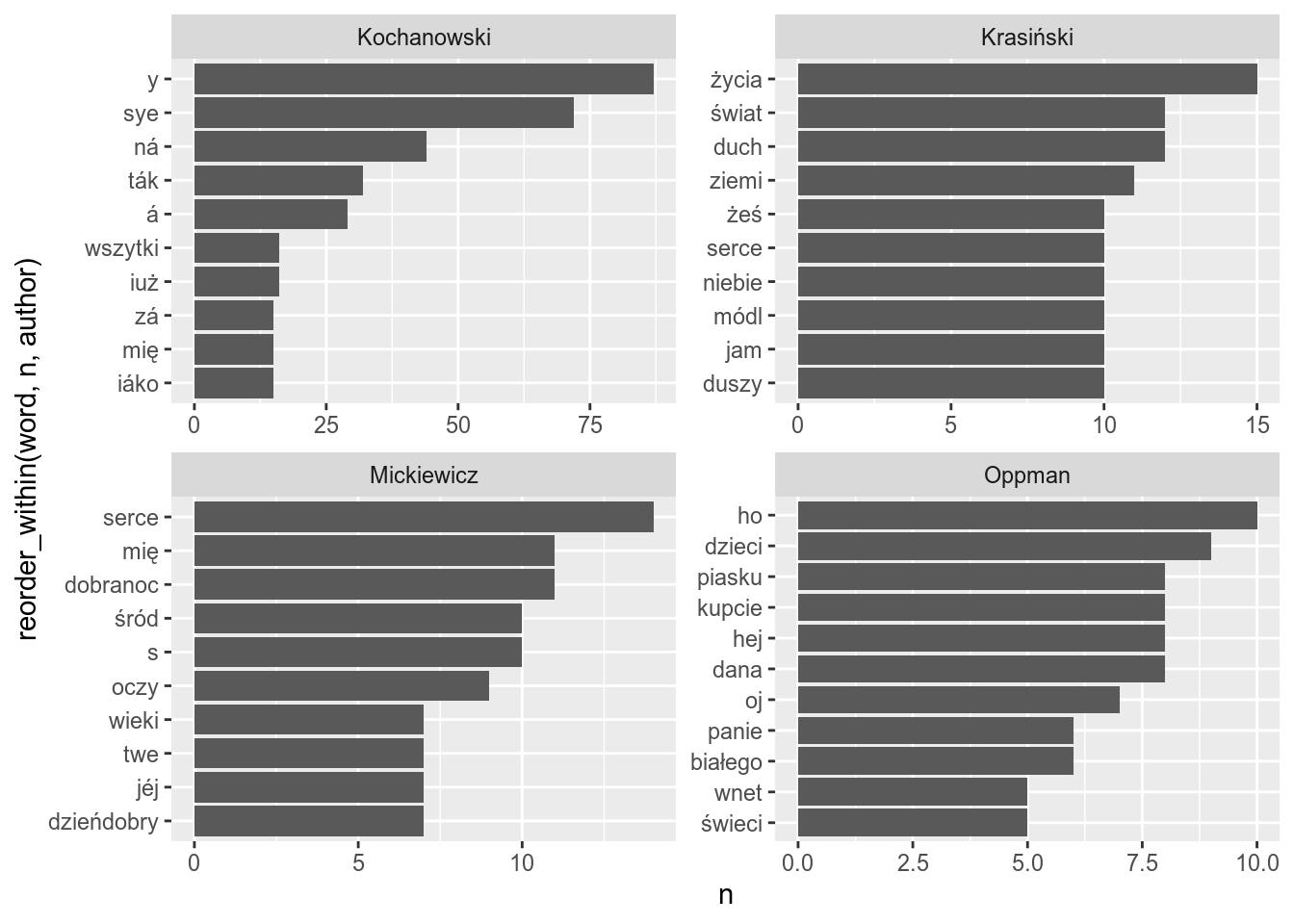
It is also possible to analyse bigrams
texts %>%
unnest_tokens(output = "bigrams", input = text, token = "ngrams", n = 2) %>%
# separate into two seperate columns each part of bigram
separate(bigrams, into = c("word_1", "word_2"), sep = " ") %>%
# filter out those that have stopwords
anti_join(tibble(word_1 = stopwords)) %>%
anti_join(tibble(word_2 = stopwords)) %>%
# merge separate columns into one
mutate(bigrams = str_c(word_1, word_2, sep = " ")) %>%
group_by(author) %>%
count(bigrams) %>%
top_n(4) %>%
ggplot(aes(reorder_within(bigrams, n, author), n))+
geom_col()+
scale_x_reordered()+
coord_flip()+
facet_wrap(~author, scales = "free")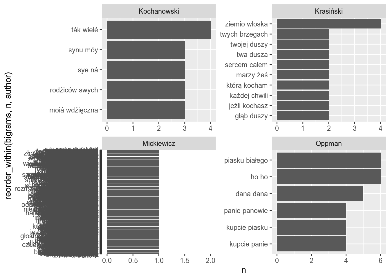
Since our corpora for each author is really small we can’t see much (e. g. Mickiewicz no repetitions). If the text will be longer (e. g. long novels), you will be able to get the most important. Lets analyse “Tajemnicę Baskerville’ów”:
tajemnica <- gutenberg_download(34079)
tajemnica %>%
unnest_tokens(output = "bigrams", input = text, token = "ngrams", n = 2) %>%
# separate into two seperate columns each part of bigram
separate(bigrams, into = c("word_1", "word_2"), sep = " ") %>%
# filter out those that have stopwords
anti_join(tibble(word_1 = stopwords)) %>%
anti_join(tibble(word_2 = stopwords)) %>%
# merge separate columns into one
mutate(bigrams = str_c(word_1, word_2, sep = " ")) %>%
count(bigrams, sort = TRUE) %>%
top_n(20) %>%
ggplot(aes(fct_reorder(bigrams, n), n))+
geom_col()+
coord_flip()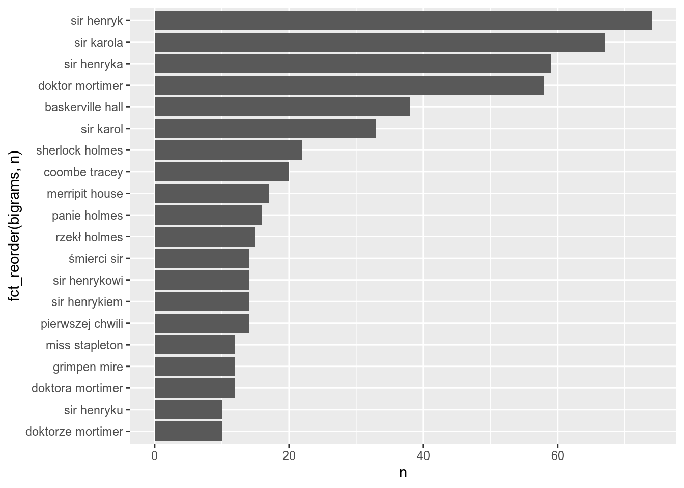
Analyse “Pan Tadeusz Czyli Ostatni Zajazd na Litwie” by A. Mickiewicz. What is the most frequent bigram in this text (remove stopwords)?
6.4 udpipe
The udpipe package gives you the ability to get lemmatisation, morphological and syntactic analysis for multiple languages. A tutorial and a list of available languages can be found here.
All models are long to download:
Texts for udpipe analyser should have variables named text and doc_id:
After you downloaded a model and created a correct dataframe it is possible to analyse our texts:
texts_parsed <- udpipe(x = texts_for_udpipe,
object = udpipe_load_model("polish-pdb-ud-2.4-190531.udpipe"))
texts_parsed
What is the most frequent part of speech (upos variable) in our corpora according to the model?
6.5 stylo
The stylo package (Eder, Rybicki, and Kestemont 2016) is a package for computational stylistics, authorship attribution, etc.
First of all it is possible to use pure frequencies as features for clustarisation:
library(stylo)
texts %>%
mutate(doc_id = str_c(author, title, sep = "_")) %>%
unnest_tokens(text, output = "word") %>%
count(doc_id, word) %>%
group_by(doc_id) %>%
mutate(ratio = n/sum(n)) %>%
pivot_wider(names_from = doc_id, values_from = ratio, values_fill = list(ratio = 0)) %>%
select(-word, -n) ->
for_stylo