1. Введение

1.1 Библиотеки

library(tidyverse)
library(ca)

1.2 Фамильная честь Вустеров

В данной лекции я буду использовать данные из романа П. Г. Вудхауза “Фамильная честь Вустеров”. В датасете собраны несколько переменных:

chapter — номер главы
гарольд — количество появлений имени в каждой из глав
гасси — количество появлений имени в каждой из глав
далия — количество появлений имени в каждой из глав
дживс — количество появлений имени в каждой из глав
мадлен — количество появлений имени в каждой из глав
оутс — количество появлений имени в каждой из глав
спод — количество появлений имени в каждой из глав
стиффи — количество появлений имени в каждой из глав
сэр — количество появлений имени в каждой из глав

wodehouse <- read.csv("https://goo.gl/bSxdMZ")
GGally::ggpairs(wodehouse[,-1])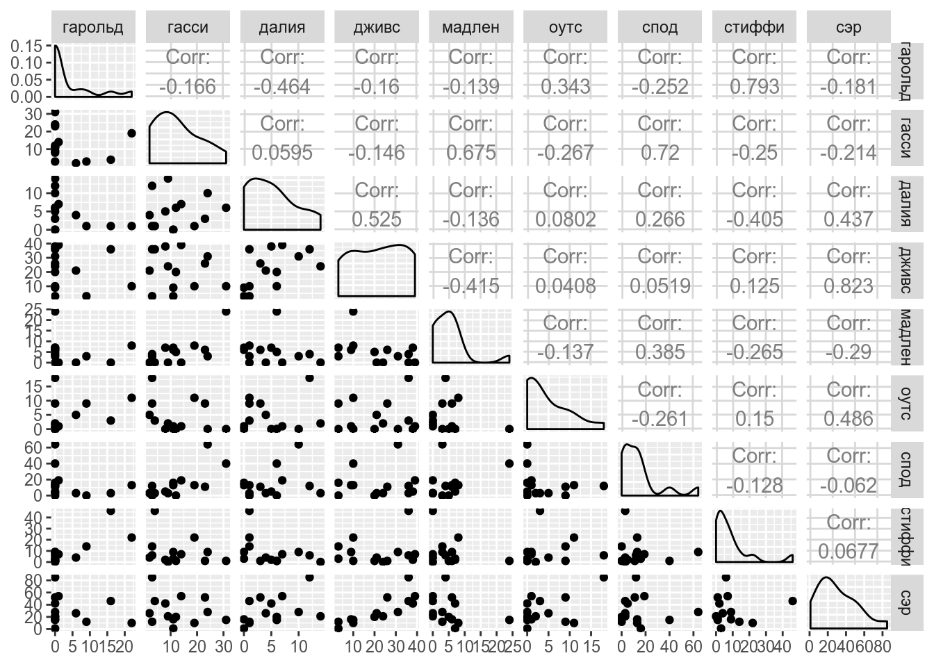

1.3 Нидерланлские каузативы

Dataset and description from paper by Natalia Levshina. Modern standard Dutch has two periphrastic causatives with the infinitive: the constructions with doen ‘do’ and laten ‘let’. The study is based on an 8-million token corpus of Netherlandic and Belgian Dutch. After the manual cleaning, there were left with 6,808 observations, which were then coded for seven semantic, syntactic, geographical and thematic variables.

Aux — a factor that specifies the causative auxiliary with levels laten and doen.
Country — a factor with levels NL (the Netherlands) and BE (Belgium).
Causation — a factor that describes the type of causation with levels Affective, Inducive, Physical and Volitional
EPTrans — a factor that specifies the transitivity of the Effected Predicate with levels Intr (intransitive) and Tr (transitive).
EPTrans1 — a factor with levels Intr and Tr. It is very similar to the previous one, except for a few observations.

dutch_caus <- read.csv("https://goo.gl/2yAR3T")

2. CA

rownames(wodehouse) <- wodehouse$chapter
ca <- ca(wodehouse[-1])
ca

## 
##  Principal inertias (eigenvalues):
##            1        2        3        4        5        6        7       
## Value      0.269248 0.208594 0.063634 0.041687 0.034383 0.012929 0.008438
## Percentage 42.07%   32.59%   9.94%    6.51%    5.37%    2.02%    1.32%   
##            8      
## Value      0.00111
## Percentage 0.17%  
## 
## 
##  Rows:
##           Глава 1  Глава 10  Глава 11  Глава 12  Глава 13  Глава 14
## Mass     0.042924  0.043595  0.087860  0.048960  0.047619  0.118042
## ChiDist  0.657319  0.503827  0.480650  0.871805  0.584273  0.664054
## Inertia  0.018546  0.011066  0.020298  0.037212  0.016256  0.052053
## Dim. 1  -0.323423 -0.420878 -0.225240 -0.223638  0.791993  0.310647
## Dim. 2  -0.829703  0.638712 -0.563479 -1.328967 -0.653949 -1.109652
##           Глава 2   Глава 3  Глава 4   Глава 5   Глава 6   Глава 7
## Mass     0.071764  0.085178 0.077800  0.095238  0.027498  0.113347
## ChiDist  0.594474  1.048459 1.064355  0.412476  1.195103  0.778320
## Inertia  0.025361  0.093633 0.088136  0.016203  0.039275  0.068663
## Dim. 1  -0.135807 -1.654098 1.093472 -0.136037 -1.654453 -1.088398
## Dim. 2  -1.034327  1.123948 1.807475 -0.718441  1.770157  0.450153
##          Глава 8  Глава 9
## Mass    0.103957 0.036217
## ChiDist 0.966054 1.246820
## Inertia 0.097019 0.056302
## Dim. 1  1.587645 1.958257
## Dim. 2  0.446586 1.232483
## 
## 
##  Columns:
##          гарольд     гасси     далия     дживс    мадлен     оутс
## Mass    0.036217  0.116700  0.046948  0.205231  0.048960 0.039571
## ChiDist 1.734289  0.641171  0.882726  0.429982  1.146279 1.162493
## Inertia 0.108933  0.047976  0.036582  0.037944  0.064332 0.053476
## Dim. 1  2.558838 -0.872498 -0.458448  0.091883 -1.191267 1.337131
## Dim. 2  2.163571  0.681049 -1.147145 -0.787378  1.304640 0.046829
##              спод   стиффи       сэр
## Mass     0.135480 0.083836  0.287056
## ChiDist  0.948004 1.145983  0.453071
## Inertia  0.121757 0.110100  0.058925
## Dim. 1  -1.422440 1.658337  0.247022
## Dim. 2   0.985778 1.331784 -0.882475

summary(ca) # extended results

## Warning in abbreviate(rnames.temp, 4): abbreviate used with non-ASCII chars

## Warning in abbreviate(rnames.temp, 4): abbreviate used with non-ASCII chars

## Warning in abbreviate(rnames.temp, 4): abbreviate used with non-ASCII chars

## Warning in abbreviate(cnames.temp, 4): abbreviate used with non-ASCII chars

## 
## Principal inertias (eigenvalues):
## 
##  dim    value      %   cum%   scree plot               
##  1      0.269248  42.1  42.1  ***********              
##  2      0.208594  32.6  74.7  ********                 
##  3      0.063634   9.9  84.6  **                       
##  4      0.041687   6.5  91.1  **                       
##  5      0.034383   5.4  96.5  *                        
##  6      0.012929   2.0  98.5  *                        
##  7      0.008438   1.3  99.8                           
##  8      0.001110   0.2 100.0                           
##         -------- -----                                 
##  Total: 0.640025 100.0                                 
## 
## 
## Rows:
##         name   mass  qlt  inr    k=1 cor ctr    k=2 cor ctr  
## 1  |  Глава1 |   43  398   29 | -168  65   4 | -379 332  30 |
## 2  | Глава10 |   44  523   17 | -218 188   8 |  292 335  18 |
## 3  | Глава11 |   88  346   32 | -117  59   4 | -257 287  28 |
## 4  | Глава12 |   49  502   58 | -116  18   2 | -607 485  86 |
## 5  | Глава13 |   48  756   25 |  411 495  30 | -299 261  20 |
## 6  | Глава14 |  118  641   81 |  161  59  11 | -507 582 145 |
## 7  |  Глава2 |   72  646   40 |  -70  14   1 | -472 631  77 |
## 8  |  Глава3 |   85  910  146 | -858 670 233 |  513 240 108 |
## 9  |  Глава4 |   78  886  138 |  567 284  93 |  826 602 254 |
## 10 |  Глава5 |   95  662   25 |  -71  29   2 | -328 633  49 |
## 11 |  Глава6 |   27  974   61 | -858 516  75 |  808 458  86 |
## 12 |  Глава7 |  113  596  107 | -565 527 134 |  206  70  23 |
## 13 |  Глава8 |  104  772  152 |  824 727 262 |  204  45  21 |
## 14 |  Глава9 |   36  868   88 | 1016 664 139 |  563 204  55 |
## 
## Columns:
##     name   mass  qlt  inr    k=1 cor ctr    k=2 cor ctr  
## 1 | гаро |   36  911  170 | 1328 586 237 |  988 325 170 |
## 2 | гасс |  117  734   75 | -453 499  89 |  311 235  54 |
## 3 | дали |   47  425   57 | -238  73  10 | -524 352  62 |
## 4 | джив |  205  712   59 |   48  12   2 | -360 699 127 |
## 5 | мадл |   49  561  101 | -618 291  69 |  596 270  83 |
## 6 | оутс |   40  357   84 |  694 356  71 |   21   0   0 |
## 7 | спод |  135  832  190 | -738 606 274 |  450 226 132 |
## 8 | стиф |   84  846  172 |  860 564 231 |  608 282 149 |
## 9 |  сэр |  287  871   92 |  128  80  18 | -403 791 224 |

wodehouse_col <- data.frame(ca$colcoord)
wodehouse_col$rows <- rownames(ca$colcoord)

wodehouse_row <- data.frame(ca$rowcoord)
wodehouse_row$rows <- rownames(ca$rowcoord)

wodehouse_col %>% 
  ggplot(aes(Dim1, Dim2, label = rows))+
  geom_text(color = "blue")+
  geom_text(data = wodehouse_row, color = "red")+
  theme_bw()+
  labs(x = "Dim1 (42.1%)",
       y = "Dim2 (32.6%)")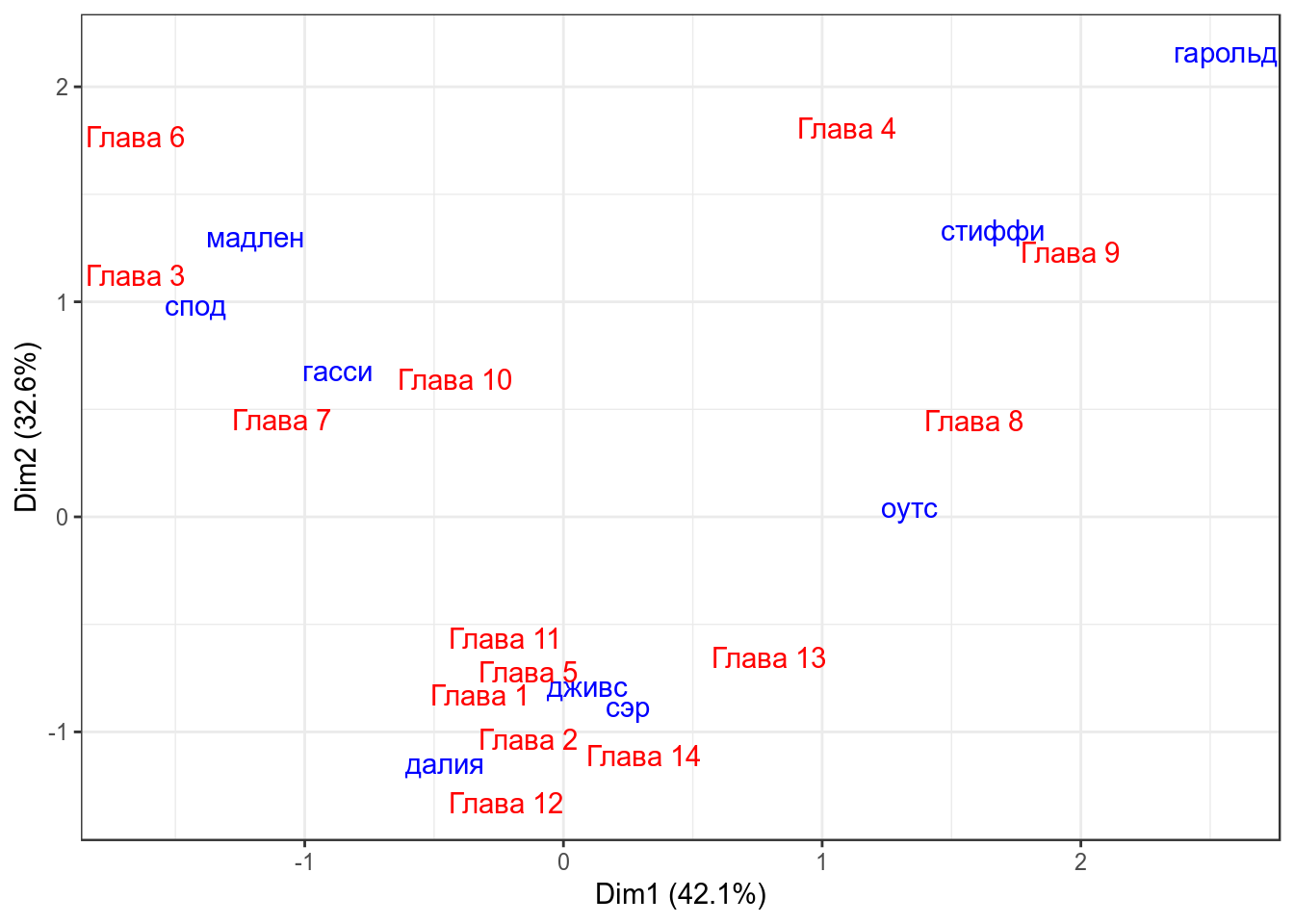

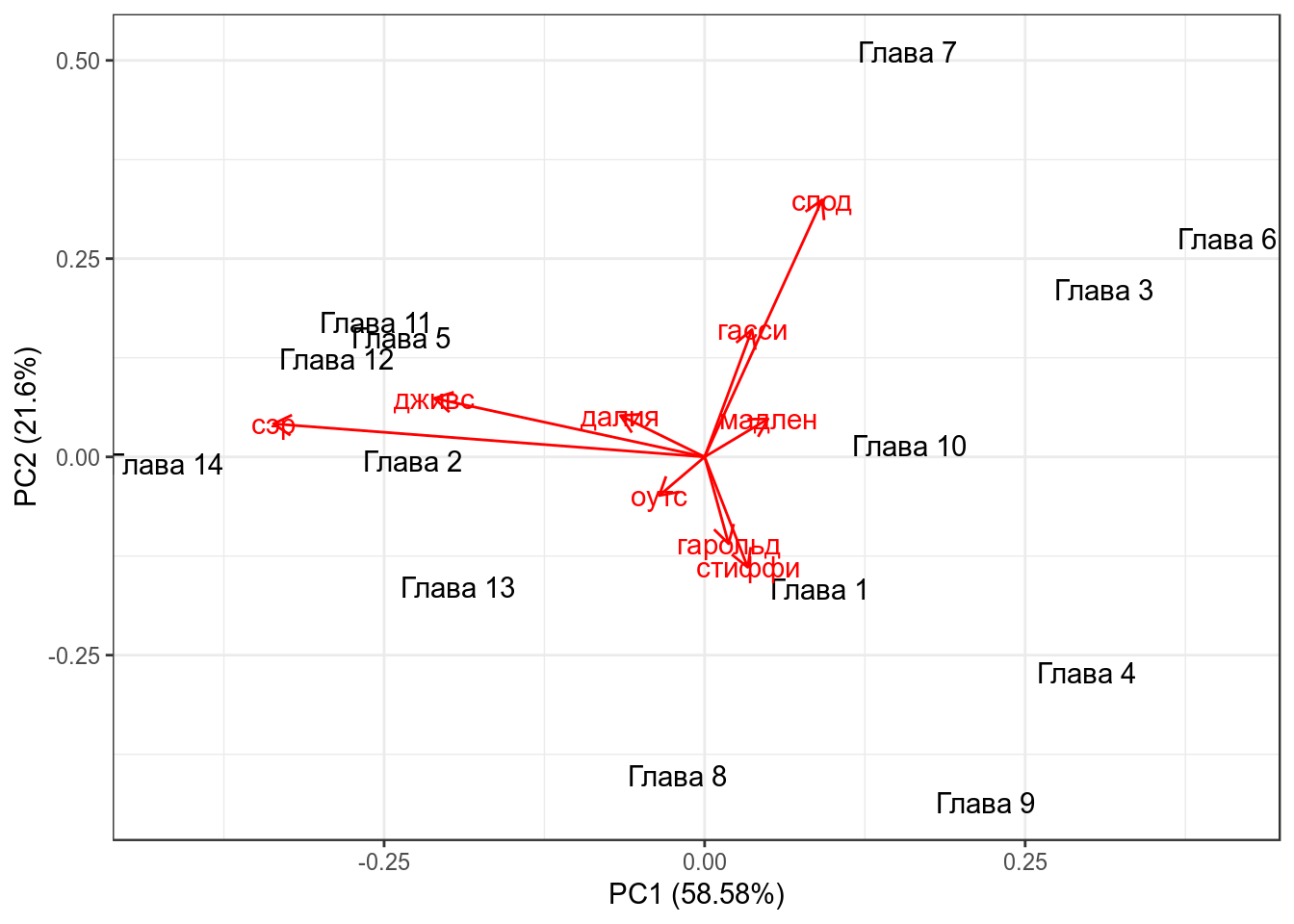
Сравните с соответствующими данными PCA:

3. MCA

MCA <- MASS::mca(dutch_caus[,-1])
MCA

## Call:
## MASS::mca(df = dutch_caus[, -1])
## 
## Multiple correspondence analysis of 500 cases of 7 factors
## 
## Correlations 0.577 0.458  cumulative % explained  9.62 17.25

dutch_caus <- cbind(dutch_caus, MCA$rs)
variables <- as_data_frame(MCA$cs)
variables$var_names <- rownames(MCA$cs)
dutch_caus %>% 
  ggplot(aes(`1`, `2`))+
  geom_point(aes(color = Aux))+
  stat_ellipse(aes(color = Aux))+
  geom_text(data = variables, aes(`1`, `2`, label = var_names))+
  theme_bw()+
  scale_x_continuous(limits = c(-0.015, 0.02))

## Warning: Removed 1 rows containing missing values (geom_text).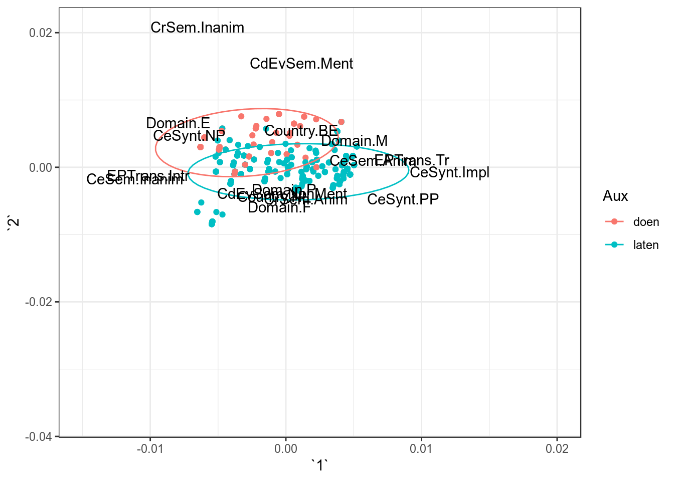

4. DCA

Комбинация CA и дискрименантного анализа называется Discriminant Correspondence Analysis.

Домашнее задание 5 (до 26.02.2019)

Домашнее задание нужно выполнять в отдельном rmarkdown файле. Получившийся файл следует помещать в соответствующую папку в своем репозитории на гитхабе. Более подробные инструкции см. на этой странице.

5.1

Скачайте датасет chairs, в котором собраны разные описания экземпляров из немецких он-лайн каталогов, отнесенным к категориям Stuhl ‘стул’ or Sessel ‘кресло’. В датасете 19 переменных:

Shop a factor that describes the online store with levels ikea.de, Moebel-Profi.de and roller.de.
WordDE a factor that describes the specific lexical category.
Category a factor that describes the more general lexical category (usually the last element of a composite noun), with levels Sessel and Stuhl.
Function a factor with levels Eat, NotSpec, Outdoor, Relax and Work.
Age a factor with levels Adult and Children.
Back a factor with levels Adjust, High, Low and Mid.
Soft a factor with levels No, Pad and Yes.
Arms a factor with levels No and Yes.
Upholst a factor with levels No and Yes.
MaterialSeat a factor with levels Fabric, Leather, Loom_natur, Metal, Paper, Plastic, Polyamide, Rattan, Steel and Wood.
SeatHeight a factor with levels Adjust, High and Norm.
SeatDepth a factor with levels Adjust, Deep and Norm.
Swivel a factor with levels No and Yes
Roll a factor with levels No and Yes.
Rock a factor with levels No and Rock.
AddFunctions a factor with levels Bed, No and Table.
Recline a factor with levels No and Yes.
ReclineBack a factor with levels No and Yes.
SaveSpace a factor with levels collapse, No and stack.

Используйте все переменные кроме переменных Shop, WordDE и Category, чтобы построить MCA. Нарисуйте все наблюдения, раскрасьте их по переменной Category и добавьте доверительные эллипсы. Сверху нанесите переменные из получившейся модели MCA. Получившийся график ggplot запустите в консоль.

5.2

Проанализируйте полученные результаты. Что Вы можете сказать на основе полученных результатов про категории Stuhl и Sessel в немецком? Что Вы можете сказать про переменные?

5.3

Cкачайте данные, содержащие 11 базовых цветов в разных подкорпусах Corpus of Contemporary American English (Davies 2008 - ). Учитывались только адъективные употребления. Постройте CA и нарисуйте биплот с переменными из столбцов и строчек (без стрелочек). Получившийся график ggplot запустите в консоль.

5.4

Проинтерпретируйте полученные результаты.

Уменьшение размерности: CA и MCA

Г. Мороз