9. Логистическая и мультиномиальная регрессия

0. Введение

Логистическая (logit, logistic) и мультиномиальная (multinomial) регрессия применяются в случаях, когда зависимая переменная является категориальной:

• с двумя значениями (логистическая регрессия)
• с более чем двумя значениями (мультиномиальная регрессия)

library(tidyverse)
library(pscl)
library(nnet)

ej_n_cons <- read.csv("https://goo.gl/DsRMve")
ej_n_cons %>% 
  ggplot(aes(ejectives, consonants, fill = ejectives, label = language))+
  geom_boxplot(show.legend = FALSE)+
  geom_jitter() +
  theme_bw() ->
  ej_n_cons_plot
plotly::ggplotly(ej_n_cons_plot, tooltip = c("label"))

marginal_verbs <- read_csv("https://goo.gl/6Phok3")

## Parsed with column specification:
## cols(
##   Gender = col_character(),
##   Age = col_double(),
##   AgeGroup = col_character(),
##   Education = col_character(),
##   City = col_character(),
##   SubjectCode = col_character(),
##   Score = col_character(),
##   GivenScore = col_double(),
##   Stimulus = col_character(),
##   Prefix = col_character(),
##   WordType = col_character(),
##   CorpusFrequency = col_double()
## )

head(marginal_verbs)

nanai <- read_csv("https://goo.gl/9uGBoQ")

## Parsed with column specification:
## cols(
##   sound = col_character(),
##   f1 = col_double(),
##   f2 = col_double()
## )

nanai %>% 
  ggplot(aes(f2, f1, label = sound, color = sound))+
  geom_text()+
  geom_rug()+
  scale_y_reverse()+
  scale_x_reverse()+
  stat_ellipse()+
  theme_bw()+
  theme(legend.position = "none")+
  labs(title = "Нанайские гласные в произнесении мужчины из селения Джуен")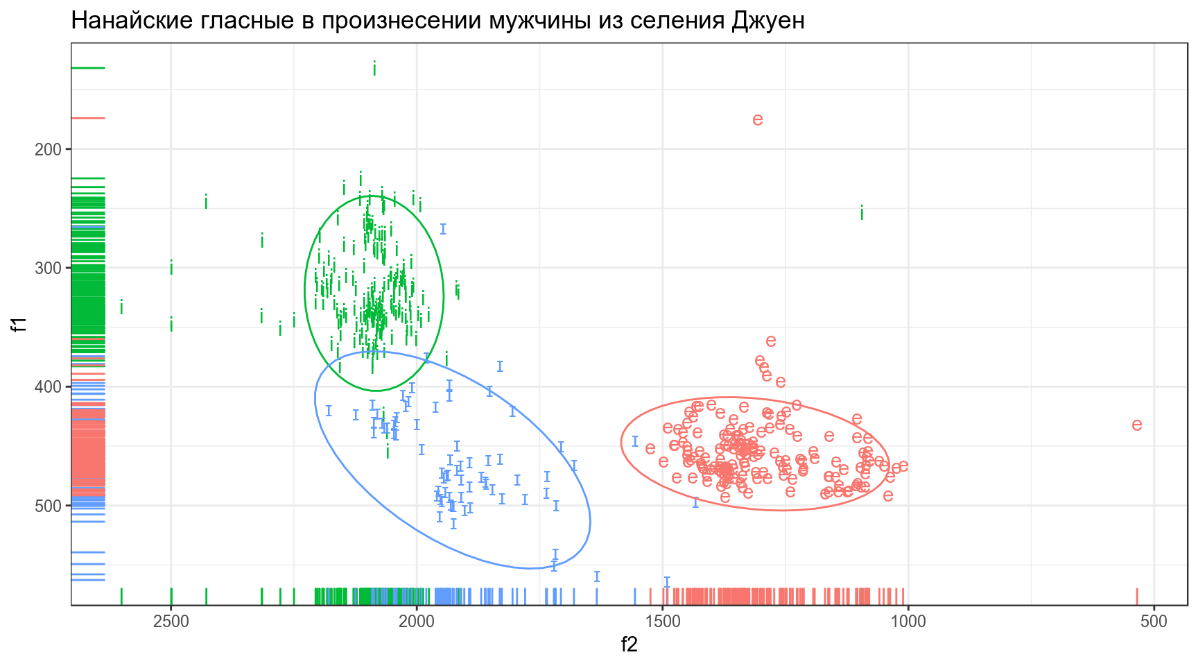

1. Логистическая регрессия

Мы хотим чего-то такого: $$\underbrace{y}_{[-\infty, +\infty]}=\underbrace{\mbox{β}_0+\mbox{β}_1\cdot x_1+\mbox{β}_2\cdot x_2 + \dots +\mbox{β}_k\cdot x_k +\mbox{ε}_i}_{[-\infty, +\infty]}$$ Вероятность — (в классической статистике) отношение количества успехов к общему числу событий: $$p = \frac{\mbox{# успехов}}{\mbox{# неудач} + \mbox{# успехов}}, \mbox{область значений: }[0, 1]$$ Шансы — отношение количества успехов к количеству неудач: $$odds = \frac{p}{1-p} = \frac{p\mbox{(успеха)}}{p\mbox{(неудачи)}}, \mbox{область значений: }[0, +\infty]$$ Натуральный логарифм шансов: $$\log(odds), \mbox{область значений: }[-\infty, +\infty]$$

Но, что нам говорит логарифм шансов? Как нам его интерпретировать?

data_frame(n = 10,
           success = 1:9,
           failure = n - success,
           prob.1 = success/(success+failure),
           odds = success/failure,
           log_odds = log(odds),
           prob.2 = exp(log_odds)/(1+exp(log_odds)))

## Warning: `data_frame()` is deprecated, use `tibble()`.
## This warning is displayed once per session.

Как связаны вероятность и логарифм шансов: $$\log(odds) = \log\left(\frac{p}{1-p}\right)$$ $$p = \frac{\exp(\log(odds))}{1+\exp(\log(odds))}$$

Как связаны вероятность и логарифм шансов:

data_frame(p = seq(0, 1, 0.001),
           log_odds = log(p/(1-p))) %>% 
  ggplot(aes(log_odds, p))+
  geom_line()+
  labs(x = latex2exp::TeX("$log\\left(\\frac{p}{1-p}\\right)$"))+
  theme_bw()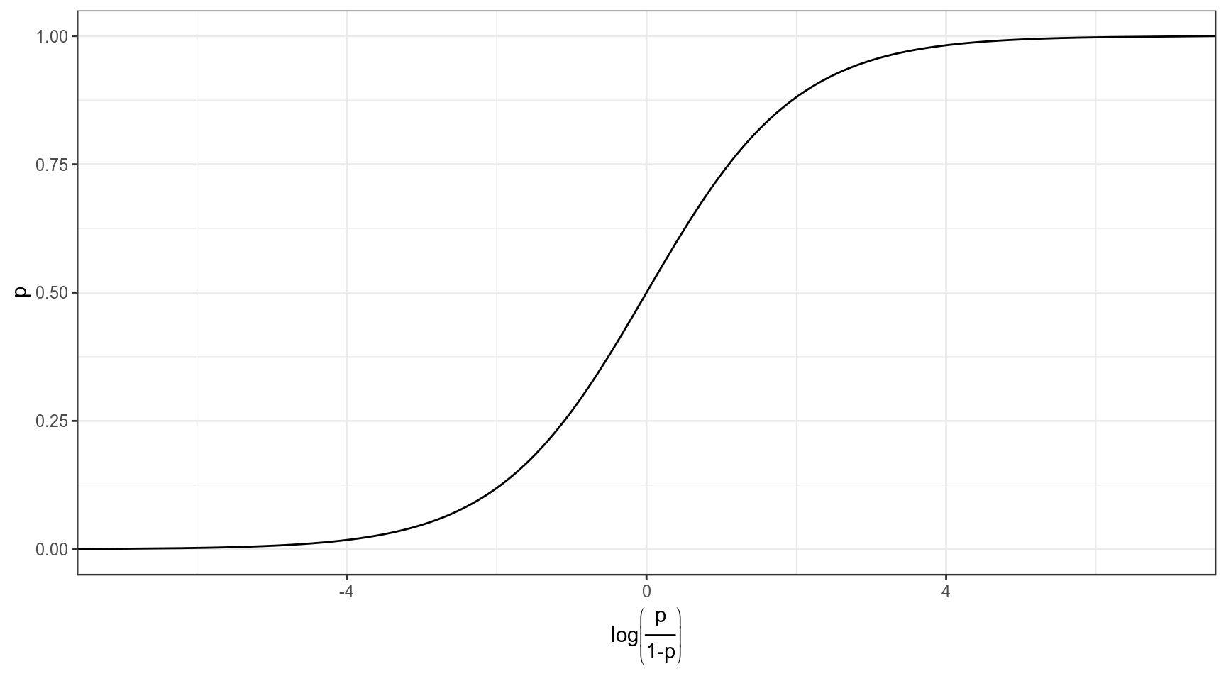

1.1 Почему не линейную регрессию?

lm_0 <- lm(as.integer(ejectives)~1, data = ej_n_cons)
lm_1 <- lm(as.integer(ejectives)~consonants, data = ej_n_cons)
lm_0

## 
## Call:
## lm(formula = as.integer(ejectives) ~ 1, data = ej_n_cons)
## 
## Coefficients:
## (Intercept)  
##       1.316

lm_1

## 
## Call:
## lm(formula = as.integer(ejectives) ~ consonants, data = ej_n_cons)
## 
## Coefficients:
## (Intercept)   consonants  
##      0.4611       0.0353

Первая модель: $$ejectives = 1.316 \times consonants$$ Вторая модель: $$ejectives = 0.4611 + 0.0353 \times consonants$$

ej_n_cons %>% 
  ggplot(aes(consonants, as.integer(ejectives)))+
  geom_point()+
  geom_smooth(method = "lm")+
  theme_bw()+
  labs(y = "ejectives (yes = 2, no = 1)")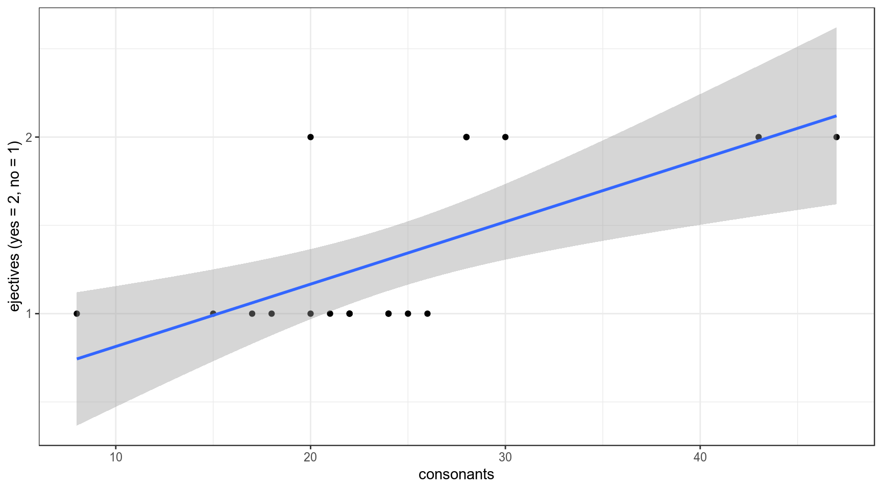

1.2 Логит: модель без предиктора

Будьте осторожны, glm не работает с тибблом.

logit_0 <- glm(ejectives~1, family = "binomial", data = ej_n_cons)
summary(logit_0)

## 
## Call:
## glm(formula = ejectives ~ 1, family = "binomial", data = ej_n_cons)
## 
## Deviance Residuals: 
##     Min       1Q   Median       3Q      Max  
## -0.8712  -0.8712  -0.8712   1.5183   1.5183  
## 
## Coefficients:
##             Estimate Std. Error z value Pr(>|z|)
## (Intercept)  -0.7732     0.4935  -1.567    0.117
## 
## (Dispersion parameter for binomial family taken to be 1)
## 
##     Null deviance: 23.699  on 18  degrees of freedom
## Residual deviance: 23.699  on 18  degrees of freedom
## AIC: 25.699
## 
## Number of Fisher Scoring iterations: 4

logit_0$coefficients

## (Intercept) 
##  -0.7731899

table(ej_n_cons$ejectives)

## 
##  no yes 
##  13   6

log(6/13) # β0

## [1] -0.7731899

6/(13+6) # p

## [1] 0.3157895

exp(log(6/13))/(1+exp(log(6/13))) # p

## [1] 0.3157895

1.3 Логит: модель c одним числовым предиктором

logit_1 <- glm(ejectives~consonants, family = "binomial", data = ej_n_cons)
summary(logit_1)

## 
## Call:
## glm(formula = ejectives ~ consonants, family = "binomial", data = ej_n_cons)
## 
## Deviance Residuals: 
##      Min        1Q    Median        3Q       Max  
## -1.08779  -0.49331  -0.20265   0.02254   2.45384  
## 
## Coefficients:
##             Estimate Std. Error z value Pr(>|z|)  
## (Intercept) -12.1123     6.1266  -1.977   0.0480 *
## consonants    0.4576     0.2436   1.878   0.0603 .
## ---
## Signif. codes:  0 '***' 0.001 '**' 0.01 '*' 0.05 '.' 0.1 ' ' 1
## 
## (Dispersion parameter for binomial family taken to be 1)
## 
##     Null deviance: 23.699  on 18  degrees of freedom
## Residual deviance: 12.192  on 17  degrees of freedom
## AIC: 16.192
## 
## Number of Fisher Scoring iterations: 6

logit_1$coefficients

## (Intercept)  consonants 
## -12.1123347   0.4576095

ej_n_cons %>% 
  mutate(ejectives = as.integer(ejectives)-1) %>% 
  ggplot(aes(consonants, ejectives)) +
  geom_point()+
  theme_bw()+
  geom_smooth(method = "glm", 
              method.args = list(family = "binomial"),
              se = FALSE)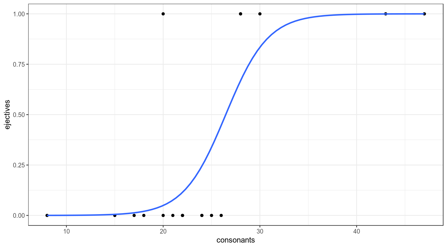

Какова вероятность, что в языке с 29 согласными есть абруптивные?

logit_1$coefficients

## (Intercept)  consonants 
## -12.1123347   0.4576095

$$\log\left({\frac{p}{1-p}}\right)_i=\beta_0+\beta_1\times consinants_i + \epsilon_i$$ $$\log\left({\frac{p}{1-p}}\right)=-12.1123347 + 0.4576095 \times 29 = 1.158341$$ $$p = \frac{e^{1.158341}}{1+e^{1.158341}} = 0.7610311$$

# log(odds)
predict(logit_1, newdata = data.frame(consonants = 29))

##        1 
## 1.158341

# p
predict(logit_1, newdata = data.frame(consonants = 29), type = "response")

##         1 
## 0.7610312

1.4 Логит: модель c одним категориальным предиктором

logit_2 <- glm(ejectives~area, family = "binomial", data = ej_n_cons)
summary(logit_2)

## 
## Call:
## glm(formula = ejectives ~ area, family = "binomial", data = ej_n_cons)
## 
## Deviance Residuals: 
##      Min        1Q    Median        3Q       Max  
## -1.66511  -0.55525  -0.00013   0.75853   1.97277  
## 
## Coefficients:
##                     Estimate Std. Error z value Pr(>|z|)
## (Intercept)        1.319e-17  1.000e+00   0.000    1.000
## areaAustralia     -1.857e+01  6.523e+03  -0.003    0.998
## areaEurasia       -1.792e+00  1.472e+00  -1.217    0.224
## areaNorth America  1.099e+00  1.528e+00   0.719    0.472
## areaPapua         -1.857e+01  6.523e+03  -0.003    0.998
## areaSouth America -1.857e+01  4.612e+03  -0.004    0.997
## 
## (Dispersion parameter for binomial family taken to be 1)
## 
##     Null deviance: 23.699  on 18  degrees of freedom
## Residual deviance: 15.785  on 13  degrees of freedom
## AIC: 27.785
## 
## Number of Fisher Scoring iterations: 17

logit_2$coefficients

##       (Intercept)     areaAustralia       areaEurasia areaNorth America 
##      1.318587e-17     -1.856607e+01     -1.791759e+00      1.098612e+00 
##         areaPapua areaSouth America 
##     -1.856607e+01     -1.856607e+01

table(ej_n_cons$ejectives, ej_n_cons$area)

##      
##       Africa Australia Eurasia North America Papua South America
##   no       2         1       6             1     1             2
##   yes      2         0       1             3     0             0

log(1/6) # Eurasia

## [1] -1.791759

log(3/1) # North America

## [1] 1.098612

1.5 Логит: множественная регрессия

logit_3 <- glm(ejectives~consonants+area, family = "binomial", data = ej_n_cons)
summary(logit_3)

## 
## Call:
## glm(formula = ejectives ~ consonants + area, family = "binomial", 
##     data = ej_n_cons)
## 
## Deviance Residuals: 
##      Min        1Q    Median        3Q       Max  
## -1.54011  -0.18623  -0.00012   0.00023   1.53307  
## 
## Coefficients:
##                     Estimate Std. Error z value Pr(>|z|)
## (Intercept)         -21.1760    15.1089  -1.402    0.161
## consonants            0.8137     0.5653   1.439    0.150
## areaAustralia       -16.2910 10754.0138  -0.002    0.999
## areaEurasia          -1.2069     3.9399  -0.306    0.759
## areaNorth America     4.0966     4.8563   0.844    0.399
## areaPapua            -4.8995 10754.0184   0.000    1.000
## areaSouth America   -17.1162  7065.6839  -0.002    0.998
## 
## (Dispersion parameter for binomial family taken to be 1)
## 
##     Null deviance: 23.6989  on 18  degrees of freedom
## Residual deviance:  6.7901  on 12  degrees of freedom
## AIC: 20.79
## 
## Number of Fisher Scoring iterations: 18

1.6 Логит: сравнение моделей

AIC(logit_0)

## [1] 25.69888

AIC(logit_1)

## [1] 16.19167

AIC(logit_2)

## [1] 27.78549

AIC(logit_3)

## [1] 20.79005

Для того, чтобы интерпретировать коэффициенты нужно проделать трансформацю:

(exp(logit_1$coefficients)-1)*100

## (Intercept)  consonants 
##   -99.99945    58.02918

Перед нами процентное изменние шансов при увеличении независимой переменной на 1.

Было предложено много аналогов R$^2$, например, McFadden’s R squared:

pscl::pR2(logit_1)

##         llh     llhNull          G2    McFadden        r2ML        r2CU 
##  -6.0958355 -11.8494421  11.5072132   0.4855593   0.4542765   0.6373812

2. Порядковая логистическая регрессия

marginal_verbs$Score <- factor(marginal_verbs$Score)
levels(marginal_verbs$Score)

## [1] "A" "B" "C" "D" "E"

ordinal <- MASS::polr(Score~Prefix+WordType+CorpusFrequency, data = marginal_verbs)
summary(ordinal)

## 
## Re-fitting to get Hessian

## Call:
## MASS::polr(formula = Score ~ Prefix + WordType + CorpusFrequency, 
##     data = marginal_verbs)
## 
## Coefficients:
##                      Value Std. Error t value
## Prefixu           0.136619  5.286e-02   2.584
## WordTypenonce     1.340603  5.693e-02  23.549
## WordTypestandard -4.655327  1.251e-01 -37.211
## CorpusFrequency  -0.001015  7.879e-05 -12.876
## 
## Intercepts:
##     Value    Std. Error t value 
## A|B  -2.6275   0.0753   -34.8784
## B|C  -1.4531   0.0552   -26.3246
## C|D  -0.2340   0.0479    -4.8853
## D|E   0.7324   0.0492    14.8986
## 
## Residual Deviance: 13138.47 
## AIC: 13154.47

ordinal$coefficients

##          Prefixu    WordTypenonce WordTypestandard  CorpusFrequency 
##      0.136619412      1.340602696     -4.655327418     -0.001014583

Как и раньше, можно преобразовать коэффициенты:

(exp(ordinal$coefficients)-1)*100

##          Prefixu    WordTypenonce WordTypestandard  CorpusFrequency 
##       14.6391763      282.1345921      -99.0489201       -0.1014068

$$\log(\frac{p(A)}{p(B|C|D|E)}) = -2.6275 + 0.136619412 \times Prefixu + 1.340602696 \times WordTypenonce -$$
$$-4.655327418 \times WordTypestandard -0.001014583\times CorpusFrequency$$ $$\log(\frac{p(A|B)}{p(C|D|E)}) = -1.4531 + 0.136619412 \times Prefixu + 1.340602696 \times WordTypenonce$$ $$-4.655327418 \times WordTypestandard -0.001014583\times CorpusFrequency$$ $$\log(\frac{p(A|B|C)}{p(D|E)}) = -0.2340 + 0.136619412 \times Prefixu + 1.340602696 \times WordTypenonce$$ $$-4.655327418 \times WordTypestandard -0.001014583\times CorpusFrequency$$ $$\log(\frac{p(A|B|C|D)}{p(E)}) = 0.7324 + 0.136619412 \times Prefixu + 1.340602696 \times WordTypenonce$$ $$-4.655327418 \times WordTypestandard -0.001014583\times CorpusFrequency$$

head(predict(ordinal))

## [1] A A E E A A
## Levels: A B C D E

head(predict(ordinal, type = "probs"))

##            A           B           C            D            E
## 1 0.99178000 0.005665533 0.001798242 0.0004683707 0.0002878525
## 2 0.93841926 0.041706786 0.013917668 0.0036817261 0.0022745617
## 3 0.06764594 0.122509282 0.252611927 0.2334448870 0.3237879649
## 4 0.01855865 0.039108932 0.113894002 0.1808984667 0.6475399508
## 5 0.90986002 0.060436871 0.020738032 0.0055351143 0.0034299624
## 6 0.91496678 0.057117954 0.019500629 0.0051963745 0.0032182669

marginal_verbs <- cbind(marginal_verbs, predict(ordinal, type = "probs"))
marginal_verbs %>%
  gather(score, predictions, A:E) %>% 
  ggplot(aes(x = score, y = predictions, fill = score)) +
  geom_col(position = "dodge")+
  facet_grid(Prefix~WordType)+
  theme_bw()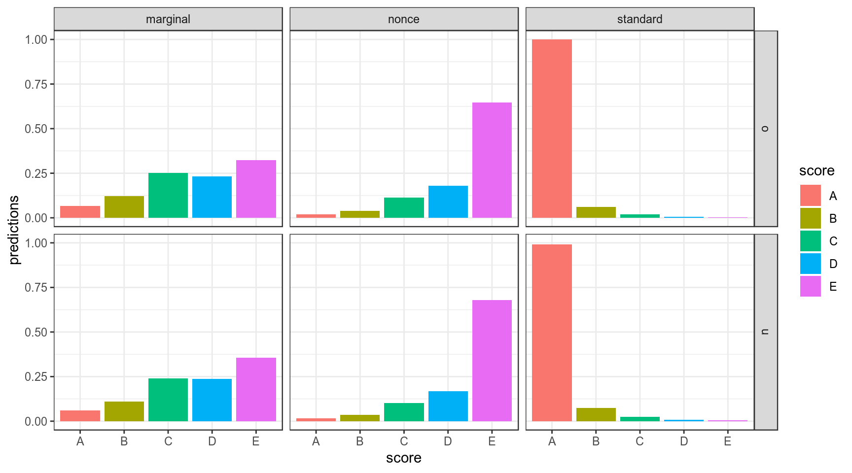

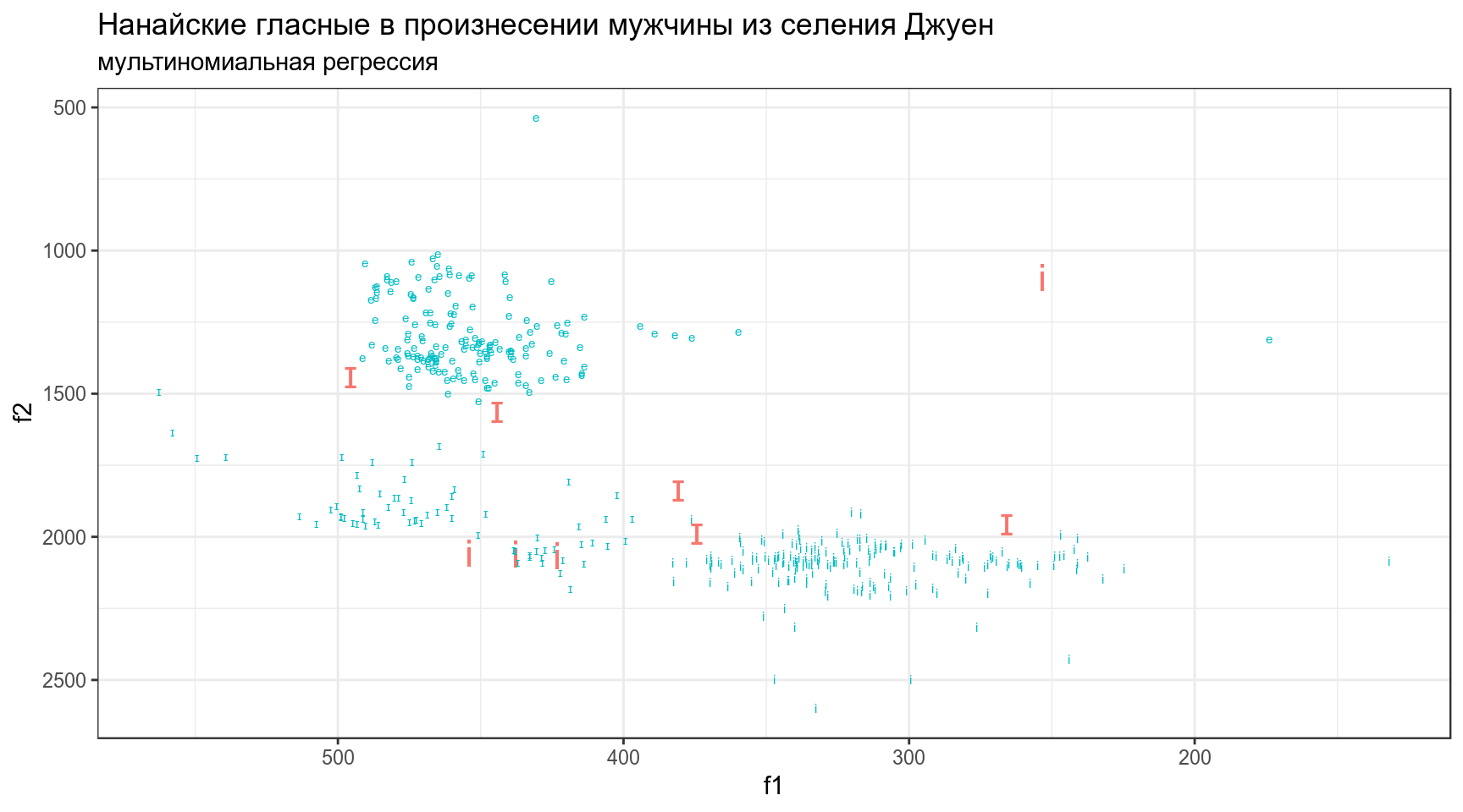
3. Мультиномиальная регрессия

mult <- nnet::multinom(sound~f1+f2, data = nanai)

## # weights:  12 (6 variable)
## initial  value 462.515774 
## iter  10 value 51.522626
## iter  20 value 46.817442
## iter  30 value 44.829080
## iter  40 value 44.807654
## iter  40 value 44.807654
## final  value 44.807654 
## converged

mult

## Call:
## nnet::multinom(formula = sound ~ f1 + f2, data = nanai)
## 
## Coefficients:
##   (Intercept)          f1         f2
## i   -22.85202 -0.04263175 0.02315226
## ɪ   -41.46147  0.02360077 0.01937067
## 
## Residual Deviance: 89.61531 
## AIC: 101.6153

$$\log(\frac{p(e)}{p(ɪ)}) = 40.88718 -0.02298543\times f1 -0.019176619\times f2$$ $$\log(\frac{p(i)}{p(ɪ)}) = 18.15078 -0.06593461\times f1 + 0.003949284\times f2$$

nanai %>% 
  mutate(prediction = predict(mult),
         correctness = sound == prediction) %>% 
  ggplot(aes(f1, f2, label = sound, color = correctness))+
  geom_text(aes(size = !correctness), show.legend = FALSE)+
  scale_y_reverse()+
  scale_x_reverse()+
  theme_bw()+
  labs(title = "Нанайские гласные в произнесении мужчины из селения Джуен",
       subtitle = "мультиномиальная регрессия")

## Warning: Using size for a discrete variable is not advised.