1. Consonants and vowels
lapsyd <- read.csv("https://goo.gl/eD4S5n")
map.feature(lapsyd$name, features = lapsyd$area,
              label = lapsyd$name,
              label.hide = TRUE)
## Warning: There is no coordinates for languages Gelao, Naxi, Nepali
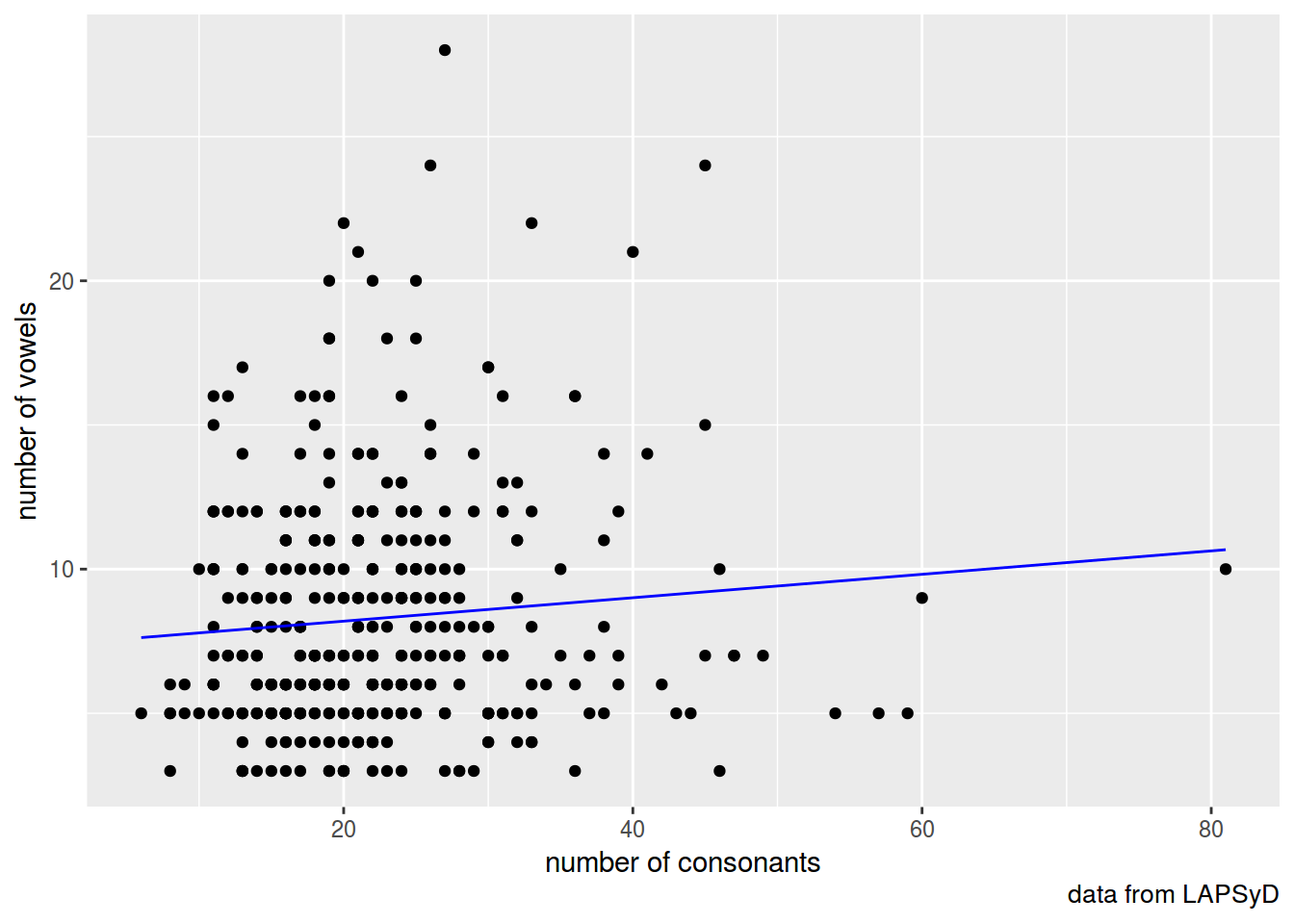
fit1 <- lm(count_vowel~count_consonant, data = lapsyd)
summary(fit1)
##
## Call:
## lm(formula = count_vowel ~ count_consonant, data = lapsyd)
##
## Residuals:
##    Min     1Q Median     3Q    Max
## -6.252 -2.992 -1.195  2.201 19.520
##
## Coefficients:
##                 Estimate Std. Error t value Pr(>|t|)
## (Intercept)      7.38236    0.54784  13.475   <2e-16 ***
## count_consonant  0.04065    0.02274   1.787   0.0746 .
## ---
## Signif. codes:  0 '***' 0.001 '**' 0.01 '*' 0.05 '.' 0.1 ' ' 1
##
## Residual standard error: 4.093 on 400 degrees of freedom
## Multiple R-squared:  0.007923,   Adjusted R-squared:  0.005443
## F-statistic: 3.195 on 1 and 400 DF,  p-value: 0.07464
lapsyd$model1 <- predict(fit1)

lapsyd %>%
  ggplot(aes(count_consonant, count_vowel))+
  geom_point()+
  geom_line(aes(count_consonant, model1), color = "blue")+
  labs(x = "number of consonants",
       y = "number of vowels",
       caption = "data from LAPSyD")
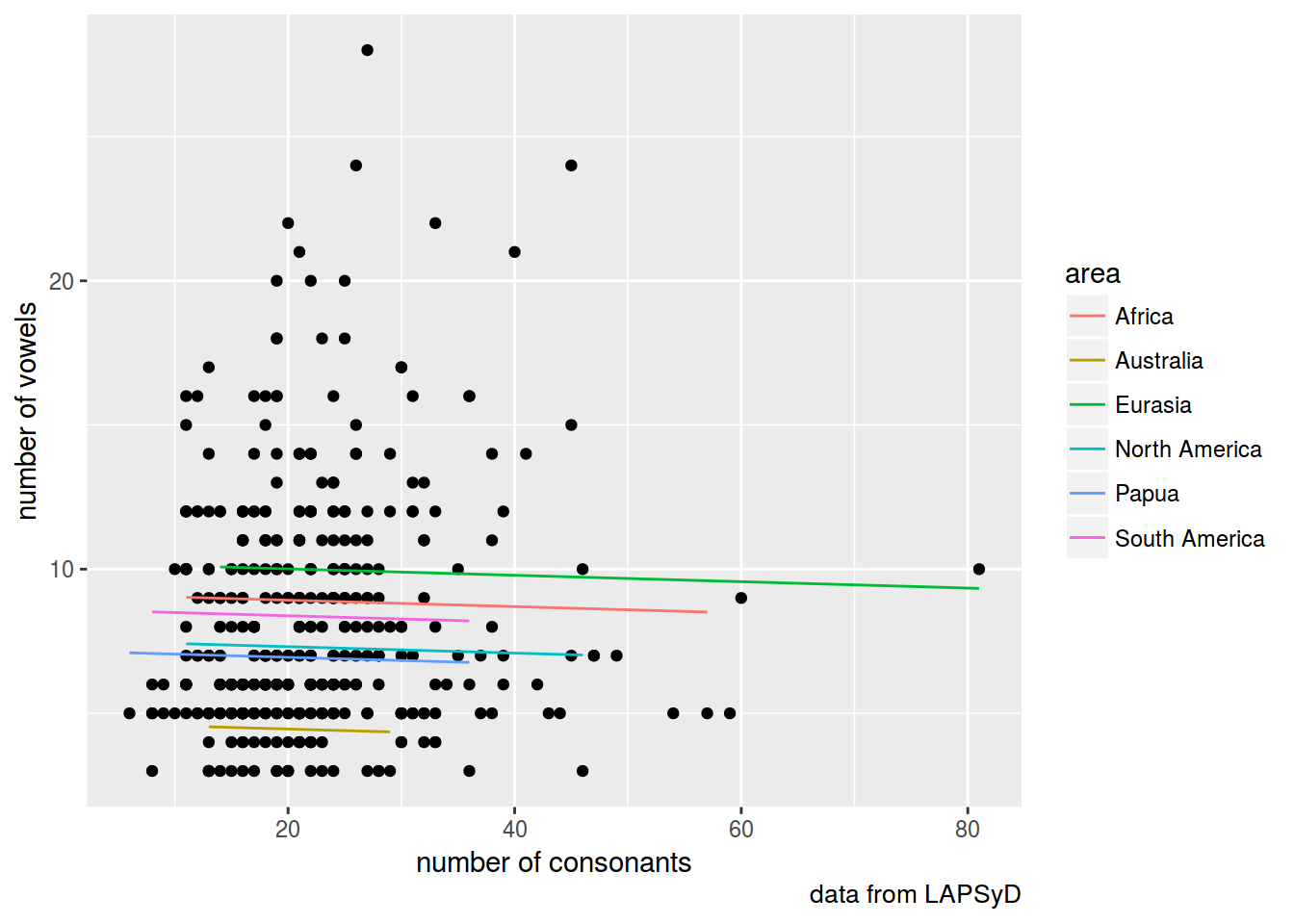
fit2 <- lmer(count_vowel ~ count_consonant + (1|area), data = lapsyd)
summary(fit2)
## Linear mixed model fit by REML ['lmerMod']
## Formula: count_vowel ~ count_consonant + (1 | area)
##    Data: lapsyd
##
## REML criterion at convergence: 2242
##
## Scaled residuals:
##     Min      1Q  Median      3Q     Max
## -1.5298 -0.6147 -0.2599  0.5146  4.7043
##
## Random effects:
##  Groups   Name        Variance Std.Dev.
##  area     (Intercept)  3.983   1.996
##  Residual             14.753   3.841
## Number of obs: 402, groups:  area, 6
##
## Fixed effects:
##                 Estimate Std. Error t value
## (Intercept)       7.8928     0.9852   8.011
## count_consonant  -0.0111     0.0240  -0.463
##
## Correlation of Fixed Effects:
##             (Intr)
## cont_cnsnnt -0.518
lapsyd$model2 <- predict(fit2)

lapsyd %>%
  ggplot(aes(count_consonant, count_vowel))+
  geom_point()+
  geom_line(aes(count_consonant, model2, color = area))+
  labs(x = "number of consonants",
       y = "number of vowels",
       caption = "data from LAPSyD")
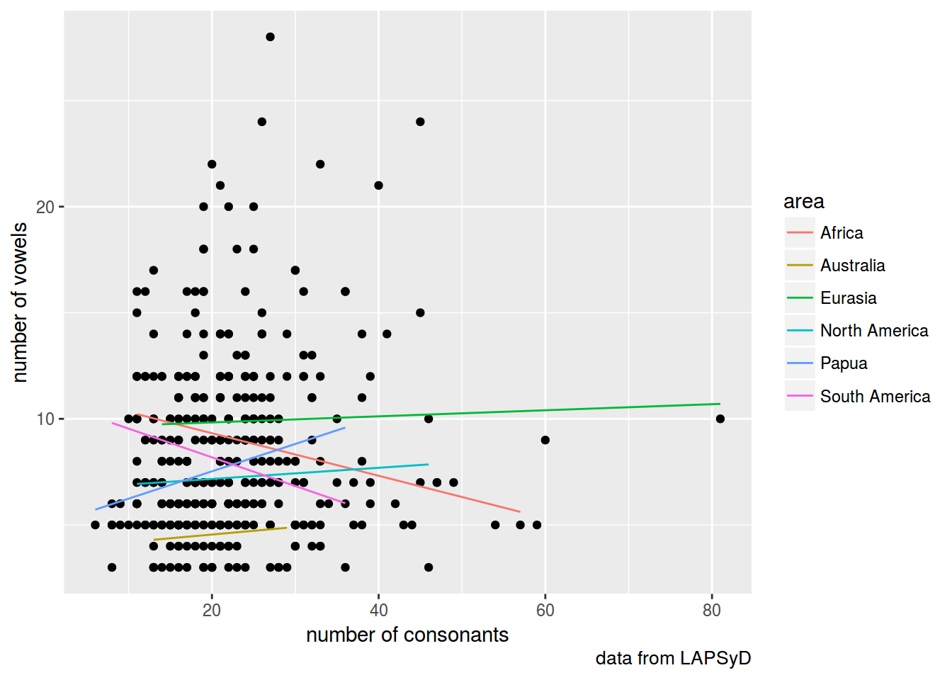
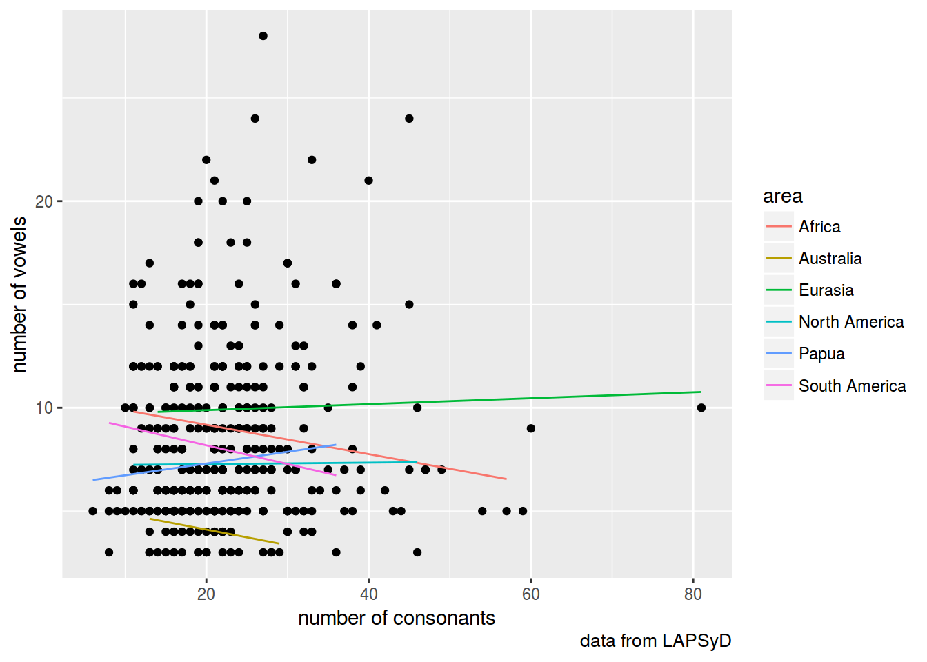
fit3 <- lmer(count_vowel ~ count_consonant + (1+count_consonant|area), data = lapsyd)
summary(fit3)
## Linear mixed model fit by REML ['lmerMod']
## Formula: count_vowel ~ count_consonant + (1 + count_consonant | area)
##    Data: lapsyd
##
## REML criterion at convergence: 2236.4
##
## Scaled residuals:
##     Min      1Q  Median      3Q     Max
## -1.7991 -0.6217 -0.2334  0.5299  4.7743
##
## Random effects:
##  Groups   Name            Variance Std.Dev. Corr
##  area     (Intercept)     11.94558 3.4562
##           count_consonant  0.01355 0.1164   -0.84
##  Residual                 14.32212 3.7845
## Number of obs: 402, groups:  area, 6
##
## Fixed effects:
##                  Estimate Std. Error t value
## (Intercept)      7.866281   1.555096   5.058
## count_consonant -0.005108   0.056987  -0.090
##
## Correlation of Fixed Effects:
##             (Intr)
## cont_cnsnnt -0.854
lapsyd$model3 <- predict(fit3)

lapsyd %>%
  ggplot(aes(count_consonant, count_vowel))+
  geom_point()+
  geom_line(aes(count_consonant, model3, color = area))+
  labs(x = "number of consonants",
       y = "number of vowels",
       caption = "data from LAPSyD")
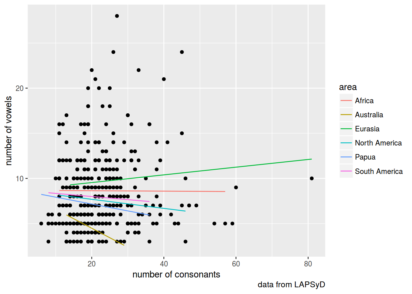
fit4 <- lmer(count_vowel ~ count_consonant + (0+count_consonant|area), data = lapsyd)
summary(fit4)
## Linear mixed model fit by REML ['lmerMod']
## Formula: count_vowel ~ count_consonant + (0 + count_consonant | area)
##    Data: lapsyd
##
## REML criterion at convergence: 2250.8
##
## Scaled residuals:
##     Min      1Q  Median      3Q     Max
## -1.5967 -0.6774 -0.2688  0.4497  4.6750
##
## Random effects:
##  Groups   Name            Variance  Std.Dev.
##  area     count_consonant  0.008151 0.09028
##  Residual                 15.093094 3.88498
## Number of obs: 402, groups:  area, 6
##
## Fixed effects:
##                 Estimate Std. Error t value
## (Intercept)      8.68579    0.59439  14.613
## count_consonant -0.05519    0.04649  -1.187
##
## Correlation of Fixed Effects:
##             (Intr)
## cont_cnsnnt -0.563
lapsyd$model4 <- predict(fit4)

lapsyd %>%
  ggplot(aes(count_consonant, count_vowel))+
  geom_point()+
  geom_line(aes(count_consonant, model4, color = area))+
  labs(x = "number of consonants",
       y = "number of vowels",
       caption = "data from LAPSyD")
fit5 <- lmer(count_vowel ~ count_consonant + (1|area) + (0+count_consonant|area), data = lapsyd)
summary(fit5)
## Linear mixed model fit by REML ['lmerMod']
## Formula:
## count_vowel ~ count_consonant + (1 | area) + (0 + count_consonant |
##     area)
##    Data: lapsyd
##
## REML criterion at convergence: 2239.8
##
## Scaled residuals:
##     Min      1Q  Median      3Q     Max
## -1.6499 -0.6023 -0.2494  0.5018  4.7428
##
## Random effects:
##  Groups   Name            Variance Std.Dev.
##  area     (Intercept)      5.67146 2.38148
##  area.1   count_consonant  0.00606 0.07785
##  Residual                 14.42645 3.79822
## Number of obs: 402, groups:  area, 6
##
## Fixed effects:
##                 Estimate Std. Error t value
## (Intercept)      8.19243    1.15107   7.117
## count_consonant -0.02700    0.04326  -0.624
##
## Correlation of Fixed Effects:
##             (Intr)
## cont_cnsnnt -0.337
lapsyd$model5 <- predict(fit5)

lapsyd %>%
  ggplot(aes(count_consonant, count_vowel))+
  geom_point()+
  geom_line(aes(count_consonant, model5, color = area))+
  labs(x = "number of consonants",
       y = "number of vowels",
       caption = "data from LAPSyD")
anova(fit5, fit4, fit3, fit2, fit1)
## refitting model(s) with ML (instead of REML)
## Data: lapsyd
## Models:
## fit1: count_vowel ~ count_consonant
## fit4: count_vowel ~ count_consonant + (0 + count_consonant | area)
## fit2: count_vowel ~ count_consonant + (1 | area)
## fit5: count_vowel ~ count_consonant + (1 | area) + (0 + count_consonant |
## fit5:     area)
## fit3: count_vowel ~ count_consonant + (1 + count_consonant | area)
##      Df    AIC    BIC  logLik deviance   Chisq Chi Df Pr(>Chisq)
## fit1  3 2277.8 2289.8 -1135.9   2271.8
## fit4  4 2254.8 2270.7 -1123.4   2246.8 25.0256      1  5.657e-07 ***
## fit2  4 2245.8 2261.8 -1118.9   2237.8  8.9793      0  < 2.2e-16 ***
## fit5  5 2246.9 2266.9 -1118.4   2236.9  0.9009      1    0.34254
## fit3  6 2245.7 2269.6 -1116.8   2233.7  3.2150      1    0.07297 .
## ---
## Signif. codes:  0 '***' 0.001 '**' 0.01 '*' 0.05 '.' 0.1 ' ' 1