1.
df <- read.csv("http://goo.gl/0btfKa")
df %>%
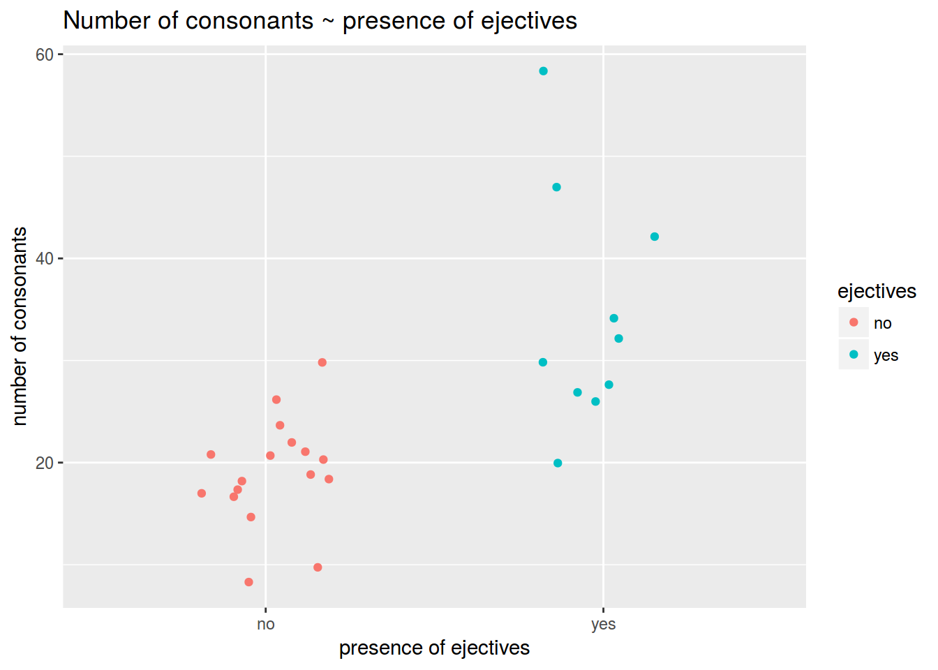
ggplot(aes(ejectives, n.cons.lapsyd, color = ejectives))+
geom_jitter(width = 0.2)+
labs(title = "Number of consonants ~ presence of ejectives",
x = "presence of ejectives",
y = "number of consonants")
df %>%
  group_by(ejectives) %>%
  summarise(mean(n.cons.lapsyd))
## # A tibble: 2 x 2
##   ejectives `mean(n.cons.lapsyd)`
##      <fctr>                 <dbl>
## 1        no              19.05882
## 2       yes              34.40000
fit <- lm(n.cons.lapsyd~ejectives, data = df)
summary(fit)
##
## Call:
## lm(formula = n.cons.lapsyd ~ ejectives, data = df)
##
## Residuals:
##     Min      1Q  Median      3Q     Max
## -14.400  -4.229  -1.059   2.441  23.600
##
## Coefficients:
##              Estimate Std. Error t value Pr(>|t|)
## (Intercept)    19.059      1.953   9.758 5.25e-10 ***
## ejectivesyes   15.341      3.209   4.780 6.59e-05 ***
## ---
## Signif. codes:  0 '***' 0.001 '**' 0.01 '*' 0.05 '.' 0.1 ' ' 1
##
## Residual standard error: 8.053 on 25 degrees of freedom
## Multiple R-squared:  0.4775, Adjusted R-squared:  0.4566
## F-statistic: 22.85 on 1 and 25 DF,  p-value: 6.588e-05
fit$coefficients
##  (Intercept) ejectivesyes
##     19.05882     15.34118
2.
df <- read.csv("https://goo.gl/7gIjvK")
df %>%
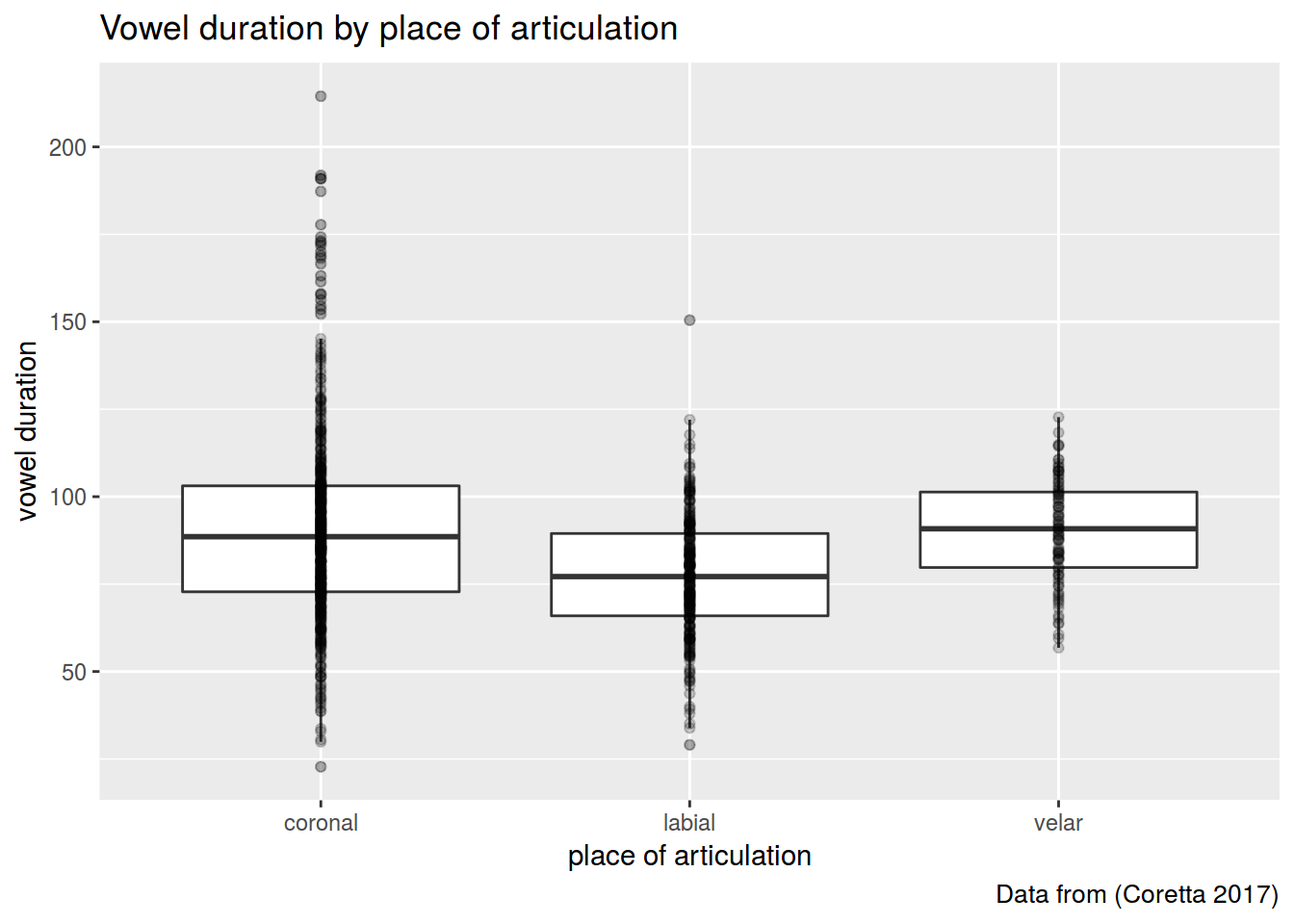
ggplot(aes(place, vowel.dur))+
geom_boxplot(outlier.alpha = 0.2)+
geom_point(alpha = 0.2)+
labs(title = "Vowel duration by place of articulation",
caption = "Data from (Coretta 2017)",
x = "place of articulation",
y = "vowel duration")
fit <- aov(vowel.dur~place, data = df)
summary(fit)
##              Df Sum Sq Mean Sq F value   Pr(>F)
## place         2  31819   15909   27.24 3.59e-12 ***
## Residuals   803 469031     584
## ---
## Signif. codes:  0 '***' 0.001 '**' 0.01 '*' 0.05 '.' 0.1 ' ' 1
fit$coefficients
## (Intercept) placelabial  placevelar
##  91.0020703 -13.7344148  -0.8073382
df %>%
  group_by(place) %>%
  summarise(mean(vowel.dur))
## # A tibble: 3 x 2
##     place `mean(vowel.dur)`
##    <fctr>             <dbl>
## 1 coronal          91.00207
## 2  labial          77.26766
## 3   velar          90.19473
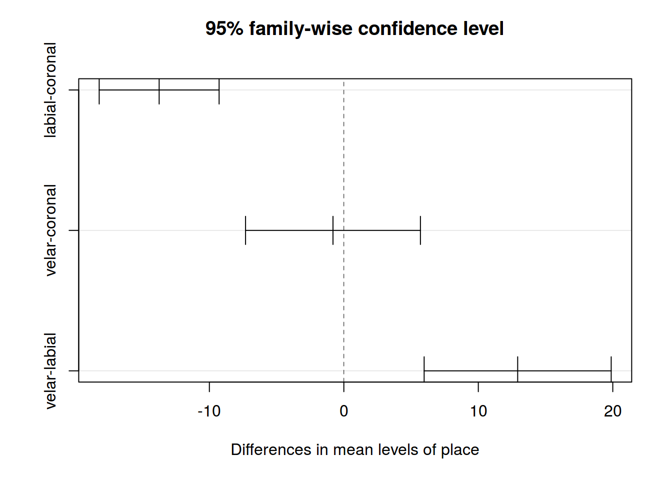
tk <- TukeyHSD(fit)
# fast visualization
plot(tk)
# ggplot
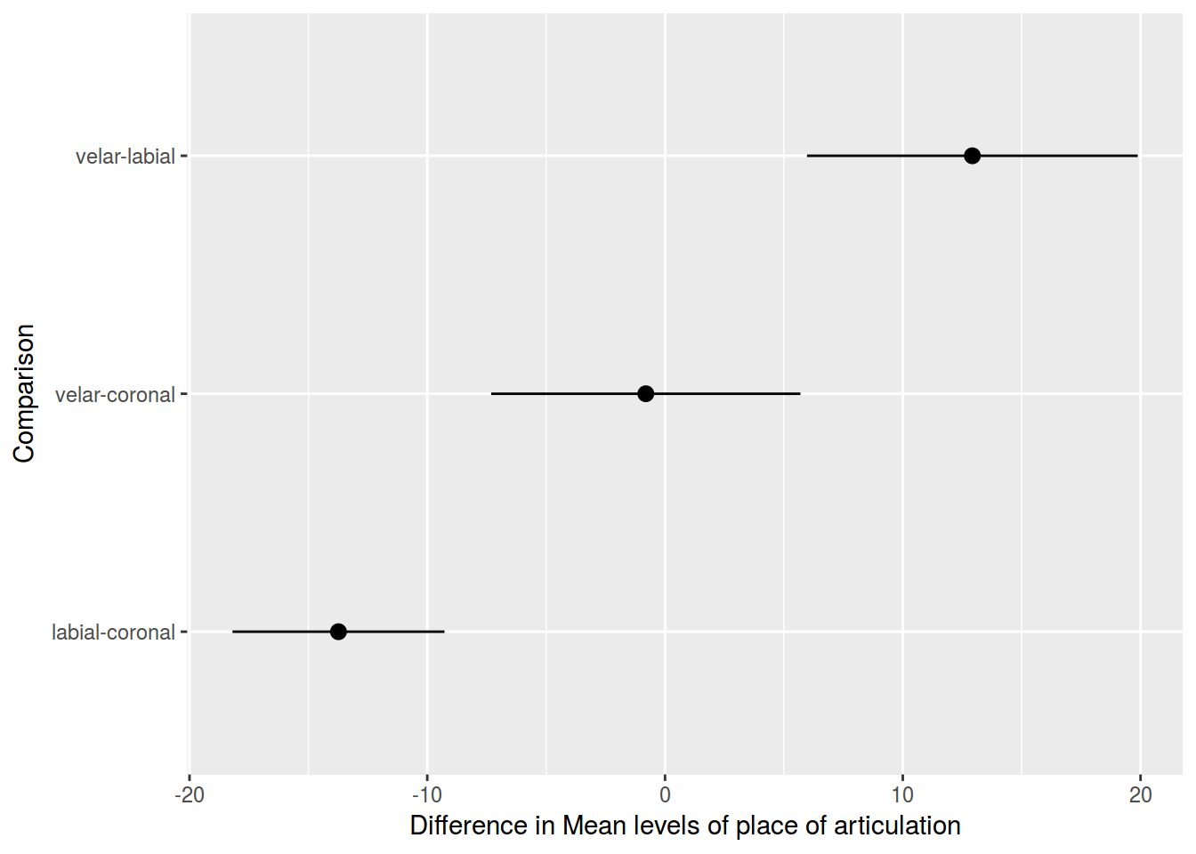
tk <- data.frame(tk$place)
tk$Comparison <- row.names(tk)
tk %>%
ggplot(aes(Comparison, y = diff, ymin = lwr, ymax = upr)) +
geom_pointrange() +
ylab("Difference in Mean levels of place of articulation") +
coord_flip()
m1 <- lm(cdi~tv.hours, data = tv)
summary(m1)
m2 <- lm(cdi~mot.education, data = tv)
summary(m2)
m3 <- lm(cdi~tv.hours+mot.education, data = tv)
summary(m3)
m4 <- lm(cdi~., data = tv[,-1])
summary(m4)
tv %>%
  ggplot(aes(tv.hours, cdi))+
  geom_smooth(method="lm")+
  geom_point()+
  facet_wrap(~tv$book.reading)