library(tidyverse)
df <- read.csv("https://goo.gl/7gIjvK")

df %>%
filter(aspiration == "yes",speaker == "tt01") %>%
select(vowel.dur) ->
asp_vowel_duration

library(bootstrap)
set.seed(42)
bootsraped_1 <- bootstrap(asp_vowel_duration$vowel.dur,
                          nboot = 1000,
                          theta = mean)
str(bootsraped_1)
## List of 5
##  $ thetastar     : num [1:1000] 77.8 81.3 79.9 75.5 77.5 ...
##  $ func.thetastar: NULL
##  $ jack.boot.val : NULL
##  $ jack.boot.se  : NULL
##  $ call          : language bootstrap(x = asp_vowel_duration$vowel.dur, nboot = 1000, theta = mean)
bootsraped_2 <- bootstrap(asp_vowel_duration$vowel.dur,
                          nboot = 1000,
                          theta = sd)
str(bootsraped_2)
## List of 5
##  $ thetastar     : num [1:1000] 16.9 15.3 14.6 17.2 21.1 ...
##  $ func.thetastar: NULL
##  $ jack.boot.val : NULL
##  $ jack.boot.se  : NULL
##  $ call          : language bootstrap(x = asp_vowel_duration$vowel.dur, nboot = 1000, theta = sd)
trimed_mean <- function(x){
  q <- quantile(x, probs = c(0.05, 0.95))
  x <- x[x > q[1] & x < q[2]]
  mean(x)
}

set.seed(42)
bootsraped_3 <- bootstrap(asp_vowel_duration$vowel.dur,
nboot = 1000,
theta = trimed_mean)
str(bootsraped_3)
## List of 5
##  $ thetastar     : num [1:1000] 77 80.9 80.5 75.4 77.4 ...
##  $ func.thetastar: NULL
##  $ jack.boot.val : NULL
##  $ jack.boot.se  : NULL
##  $ call          : language bootstrap(x = asp_vowel_duration$vowel.dur, nboot = 1000, theta = trimed_mean)
df %>%
  filter(speaker == "tt01") %>%
  select(vowel.dur, aspiration) ->
  vowel_duration

library(mosaic)

set.seed(42)
do(1000) * (
  vowel_duration %>%
    mutate(vowel.dur = shuffle(vowel.dur)) %>%
    group_by(aspiration) %>%
    summarise(mean_value = mean(vowel.dur))) ->
  many.shuffles

tail(many.shuffles)
## # A tibble: 6 x 4
##   aspiration mean_value  .row .index
##       <fctr>      <dbl> <int>  <dbl>
## 1         no   91.08676     1    998
## 2        yes   87.66137     2    998
## 3         no   88.88635     1    999
## 4        yes   89.83677     2    999
## 5         no   90.55649     1   1000
## 6        yes   88.18561     2   1000
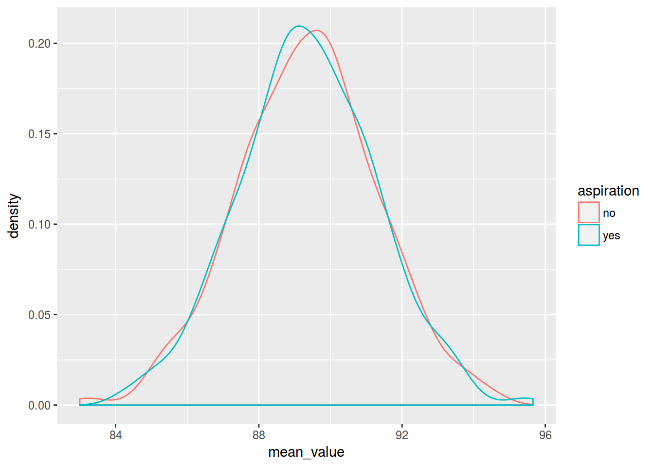
many.shuffles %>%
  ggplot(aes(mean_value, color = aspiration))+
  geom_density(alpha = 0.5)
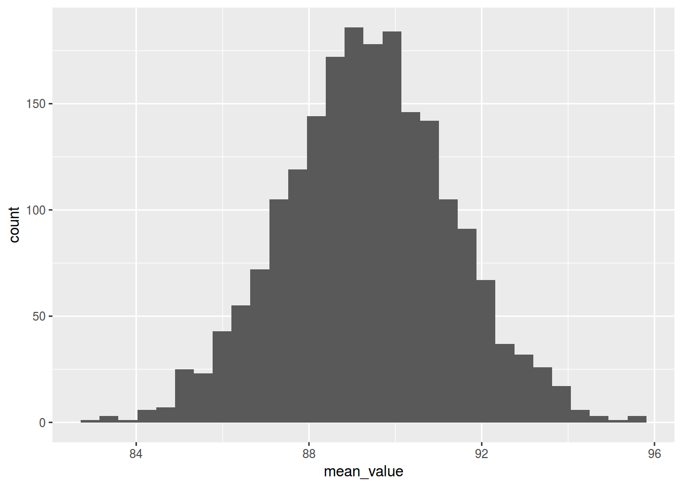
many.shuffles %>%
  ggplot(aes(mean_value))+
  geom_histogram()