Lab 7: linear regression

1.1

df <- read.csv("http://goo.gl/Qo3Yy2")

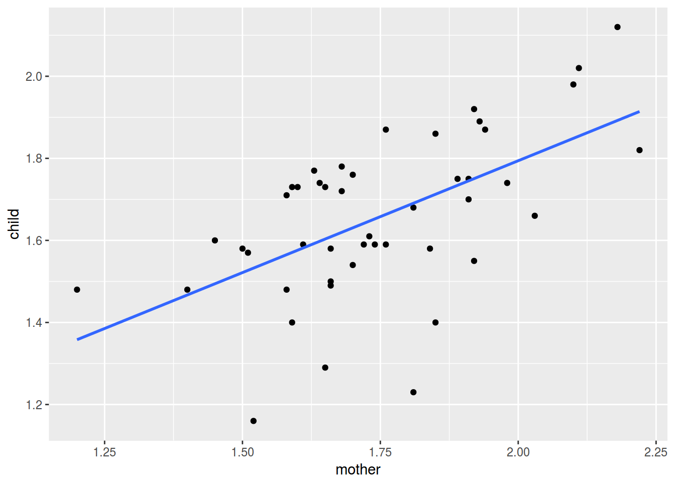
df %>%
  ggplot(aes(mother, child))+
  geom_point()+
  geom_smooth(method = "lm", se = FALSE)

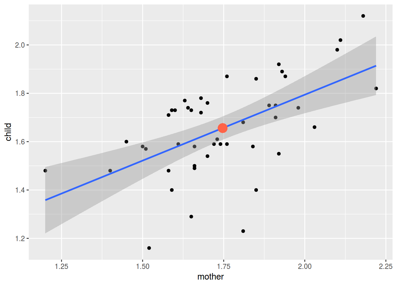
df %>%
  ggplot(aes(mother, child))+
  geom_point()+
  geom_smooth(method = "lm")+
  geom_point(aes(mean(mother), mean(child)), color = "tomato", size = 5)

cor(df)

##            child    mother
## child  1.0000000 0.5761599
## mother 0.5761599 1.0000000

fit <- lm(child~mother, data = df)
summary(fit)

## 
## Call:
## lm(formula = child ~ mother, data = df)
## 
## Residuals:
##      Min       1Q   Median       3Q      Max 
## -0.46058 -0.08925  0.01071  0.13333  0.22770 
## 
## Coefficients:
##             Estimate Std. Error t value Pr(>|t|)    
## (Intercept)   0.7038     0.2051   3.432  0.00132 ** 
## mother        0.5452     0.1166   4.676 2.79e-05 ***
## ---
## Signif. codes:  0 '***' 0.001 '**' 0.01 '*' 0.05 '.' 0.1 ' ' 1
## 
## Residual standard error: 0.1627 on 44 degrees of freedom
## Multiple R-squared:  0.332,  Adjusted R-squared:  0.3168 
## F-statistic: 21.86 on 1 and 44 DF,  p-value: 2.789e-05

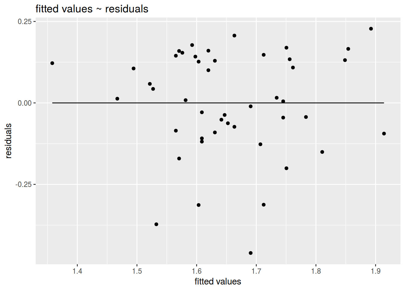
ggplot(data = fit, aes(fit$fitted.values, fit$residuals))+
  geom_point()+
  geom_line(aes(y = 0))+
  labs(title = "fitted values ~ residuals",
       x = "fitted values",
       y = "residuals")

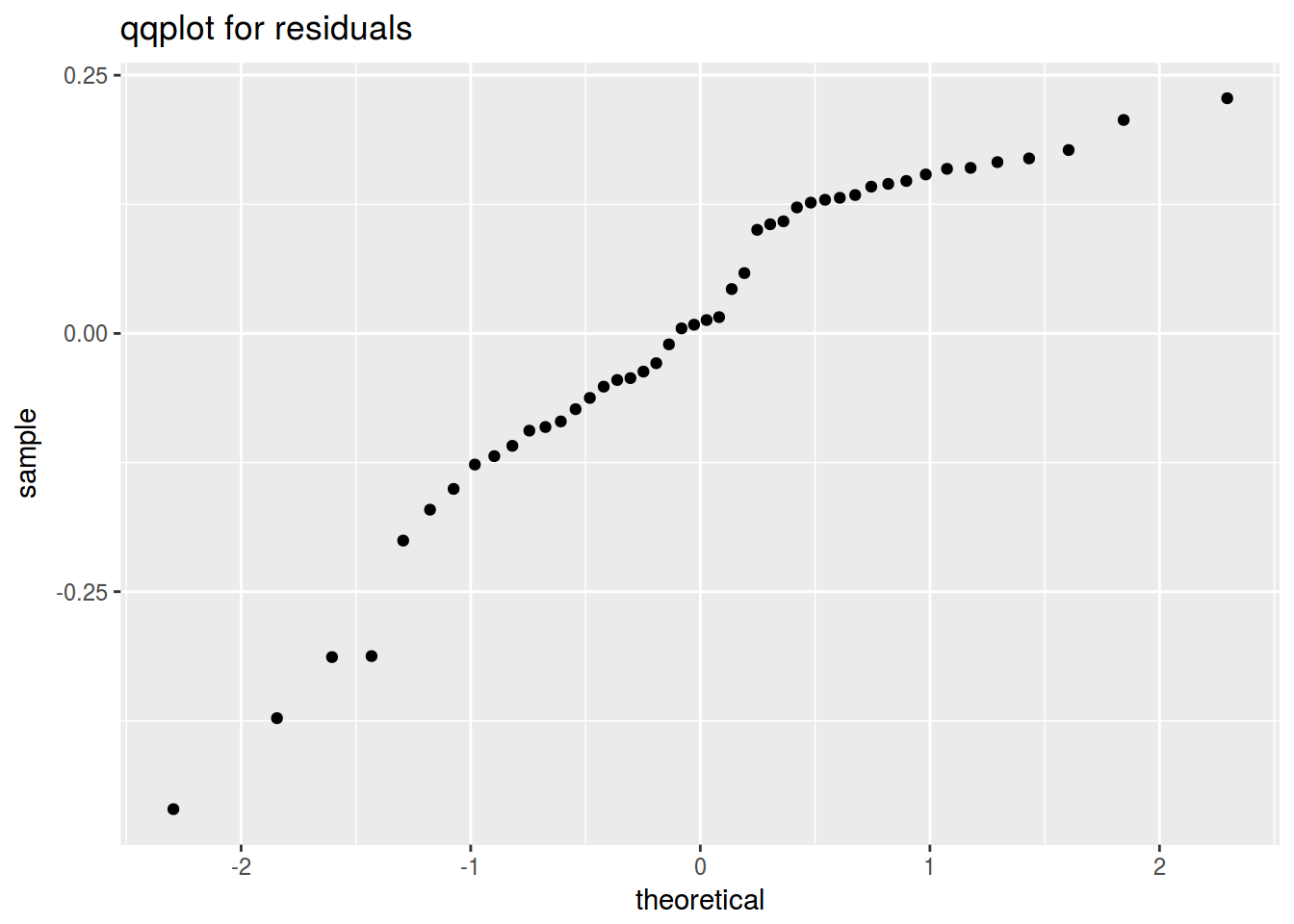
ggplot(data = fit, aes(sample = fit$residuals))+
  geom_qq()+
  labs(title = "qqplot for residuals")

predict(fit, data.frame(mother = 11:17/10))

##        1        2        3        4        5        6        7 
## 1.303490 1.358009 1.412528 1.467048 1.521567 1.576086 1.630605

2.

df <- read.csv("https://goo.gl/TcyiRc", sep = "\t")

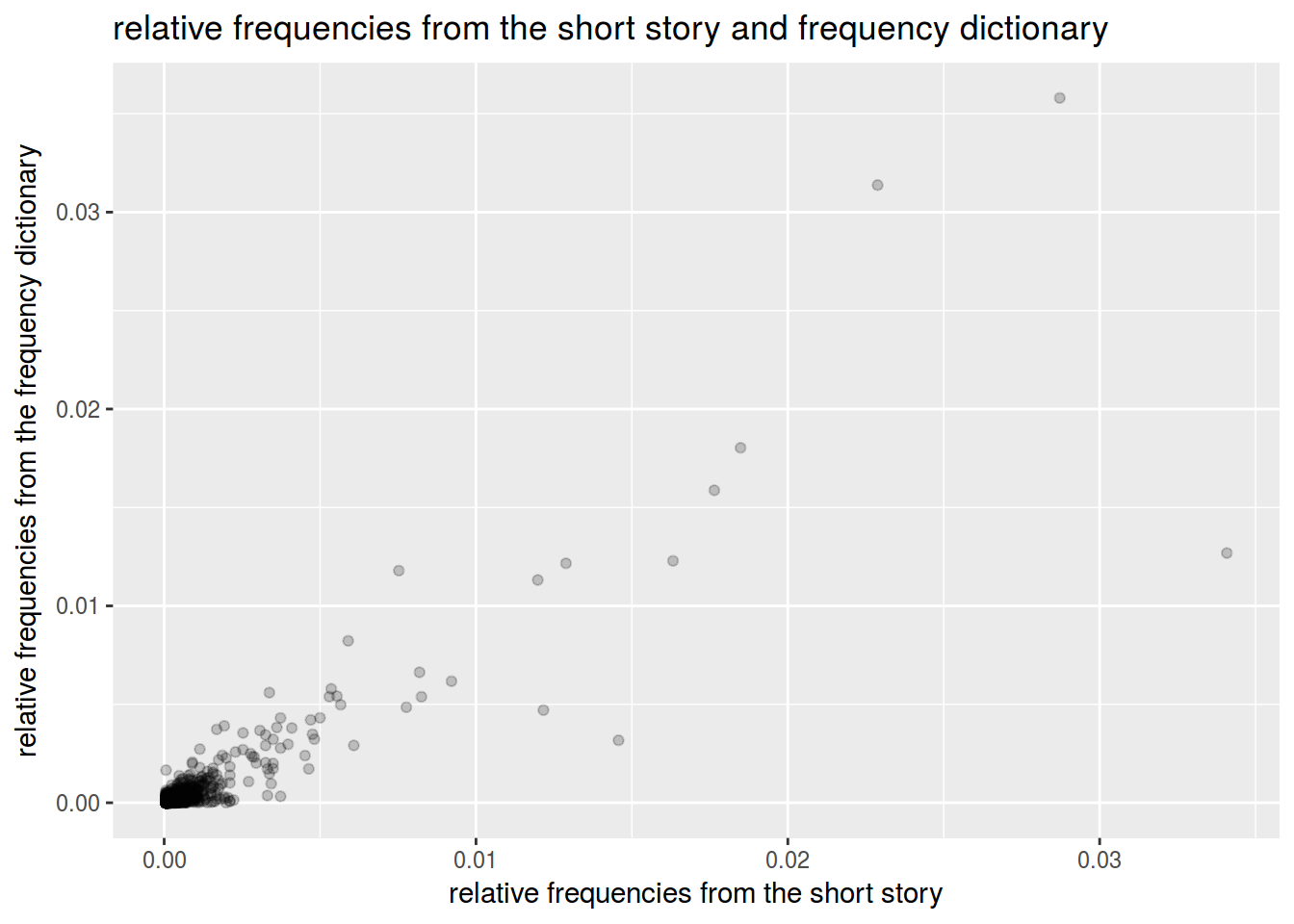
df %>% 
  ggplot(aes(r.frequency,rus.freq.dict))+
  geom_point(alpha = 0.2)+
  labs(titles = "relative frequencies from the short story and frequency dictionary",
       x = "relative frequencies from the short story",
       y = "relative frequencies from the frequency dictionary")

library(scales)
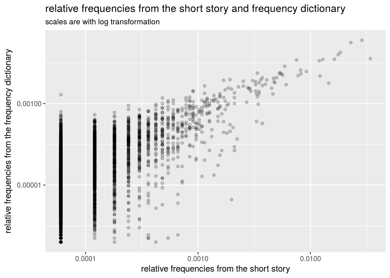
df %>% 
  ggplot(aes(r.frequency,rus.freq.dict))+
  geom_point(alpha = 0.2)+
    labs(titles = "relative frequencies from the short story and frequency dictionary",
         subtitle = "scales are with log transformation",
       x = "relative frequencies from the short story",
       y = "relative frequencies from the frequency dictionary")+
  scale_x_log10(labels = comma)+
  scale_y_log10(labels = comma)

Remark on R formula syntax

• y~x gives you \(y_i=\beta_0+\beta_1\times x_i\)
• y~x+z gives you \(y_i=\beta_0+\beta_1\times x_i+\beta_2\times z_i\)
• y~. gives you \(y_i=\beta_0+\beta_1\times x_i \dots \beta_k\times z_i\) (it makes a regression from all \(k\) predictors)
• y~1 gives you \(y_i=\beta_0\)
• y~x-1 gives you \(y_i=\beta_1\times x_i\)
• y~I(x-1) gives you \(y_i=\beta_0+\beta_1\times (x_i-1)\)
• y~I(x^2) gives you \(y_i=\beta_0+\beta_1\times x_i^2\)