Descriptive statistics. Measures of central tendency. Confidence intervals. P-value. T-test

Measures of central tendency

• (arithmetic) mean
• median
• quartiles
• mode

# Basic R:
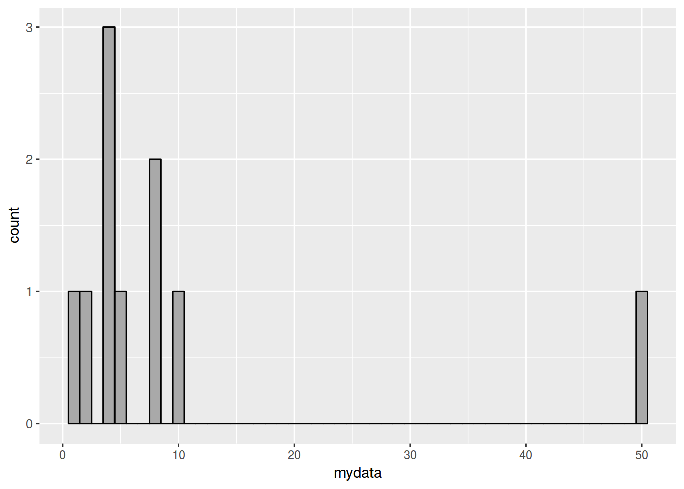
mydata <- c(1,2,4,4,4,5,8,8,10,50)
mean(mydata)

## [1] 9.6

median(mydata)

## [1] 4.5

table(mydata)

## mydata
##  1  2  4  5  8 10 50 
##  1  1  3  1  2  1  1

which.max(table(mydata))

## 4 
## 3

library(tidyverse)

data.frame(mydata) %>% 
ggplot(aes(mydata)) + 
  geom_histogram(binwidth=1, colour="black", fill="darkgray")

Standard deviation

If \(\bar{x}\) is a mean of X { x₁, x₂, x₃,… x_n } then we can calculate the difference between each point and the mean and take a sum of the squared diffs (which is called variance).

\[var = ( x_1 - \bar{x} )^2 + ( x_2 - \bar{x} )^2 + ( x_3 - \bar{x} )^2 + ... + ( x_n - \bar{x} )^2\] Standard deviation is equal to the square root of the variance (is calculated in the same units as \(x_1\)…\(x_n\)). \[sd = \sqrt{var}\]

sd(mydata)

## [1] 14.46989

mtcars data

head(mtcars$mpg) # miles per gallon

## [1] 21.0 21.0 22.8 21.4 18.7 18.1

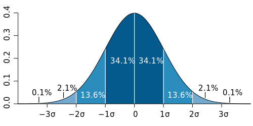
Standard deviation diagram for a normally distributed data (source: Wikipedia)

Confidence Interval

Main question: based on a given sample, what can we infer about the population?
If we have just a single sample, perhaps the best estimate of the average value would be the sample mean, usually denoted as \(\bar{x}\) (pronounced as x_bar). If we take more samples, their mean would differ a little (or a lot). So, the question is, how uncertain we are of that point estimate. For example, we would like to be 95% sure that the mean of any taken sample will be within certain interval.
For a known standard deviation, \[CI_{95\%} = \bar{x} \pm 1.96*\frac{sd}{\sqrt{n}}\] given that the values in X are randomly distributed and independent of each other.

Thus, we can say that there is only a 5% chance that the confidence interval excludes the mean of the population.
CI can be shown at different confidence levels, for example 90%, 95% and 99%. The coefficients for the calcuating CI are the following: 1.645 for 90% CI, 1.96 for 95%, 2.326 for 98% CI, 2.576 for 99% CI.

unique(mtcars$vs) # vs is either V-engine or Straight-engine

## [1] 0 1

mtcars %>%
  group_by(vs) %>%
  summarise(mean.mpg = mean(mpg, na.rm = TRUE),
            sd.mpg = sd(mpg, na.rm = TRUE),
            n.mpg = n()) %>%
  mutate(se.mpg = sd.mpg / sqrt(n.mpg),
         lower.ci.mpg = mean.mpg - qt(1 - (0.05 / 2), n.mpg - 1) * se.mpg,
         upper.ci.mpg = mean.mpg + qt(1 - (0.05 / 2), n.mpg - 1) * se.mpg)

## # A tibble: 2 × 7
##      vs mean.mpg   sd.mpg n.mpg    se.mpg lower.ci.mpg upper.ci.mpg
##   <dbl>    <dbl>    <dbl> <int>     <dbl>        <dbl>        <dbl>
## 1     0 16.61667 3.860699    18 0.9099756     14.69679     18.53655
## 2     1 24.55714 5.378978    14 1.4375924     21.45141     27.66287